Homework 1 - Bias-Variance Tradeoff and Linear Regression

Due Friday, Feb 9 11:59 PM

• Please submit your work in one PDF file to D2L > Assessments > Dropbox. Multiple files or a file that is not in pdf format are not allowed.

• Any relevant code should be attached.

• Read ISL Chapter 2 and 3.

Homework Questions

1. ISL Sec. 2.4: 3

2. ISL Sec. 2.4: 6

3. ISL Sec. 3.7: 4

4. ISL Sec. 3.7: 5

5. ISL Sec. 3.7: 6

6. ISL Sec. 3.7: 14

7. Simulation of bias-variance tradeoff. Let \(f(x) = x ^ 2\) be the true regression function. Simulate the data using \(y_i = f(x_i) + \epsilon_i, i = 1, \dots, 100\), where \(x_i = 0.01i\) and \(\epsilon_i \stackrel{iid} \sim N(0, 0.3^2).\)

   1. Generate 250 training data sets.
   2. For each data set, fit the following three models:
   • Model 1: \(y = \beta_0+\beta_1x+\epsilon\)
   • Model 2: \(y = \beta_0+\beta_1x+ \beta_2x^2 + \epsilon\)
   • Model 3: \(y = \beta_0+\beta_1x+ \beta_2x^2 + \cdots + \beta_9x^9 + \epsilon\)
   3. Calculate empirical MSE of \(\hat{f}\), bias of \(\hat{f}\) and variance of \(\hat{f}\). Then show that \[\text{MSE}_{\hat{f}} \approx \text{Bias}^2(\hat{f}) + \mathrm{Var}(\hat{f}).\] Specifically, for each value of \(x_i\), \(i = 1, \dots, 100\),

   \[\text{MSE}_{\hat{f}} = \frac{1}{250}\sum_{k=1}^{250} \left(\hat{f}_k(x_i) - f(x_i) \right) ^2,\] \[\text{Bias}(\hat{f}) = \overline{\hat{f}}(x_i) - f(x_i),\] where \(\overline{\hat{f}}(x_i) = \frac{1}{250}\sum_{k = 1}^{250}\hat{f}_k(x_i)\) is the sample mean of \(\hat{f}(x_i)\) that approximates \(\mathrm{E}_{\hat{f}}\left(\hat{f}(x_i)\right).\) \[ \mathrm{Var}(\hat{f}) = \frac{1}{250}\sum_{k=1}^{250} \left(\hat{f}_k(x_i) - \overline{\hat{f}}(x_i) \right) ^2.\] [Note:] If you calculate the variance using the built-in function such as 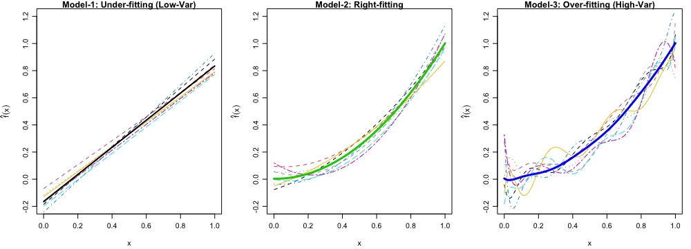var() in R, the identity holds only approximately because of the \(250 - 1\) term in the denominator in the sample variance formula. If instead \(250\) is used in the denominator, the identity holds exactly.

   4. For each model, plot first ten estimated \(f\), \(\hat{f}_{1}(x), \dots, \hat{f}_{10}(x)\), and the average of \(\hat{f}\), \(\frac{1}{250}\sum_{k=1}^{250}\hat{f}_{k}(x)\) in one figure, as Figure 1 below. What’s your finding?
   5. Generate one more data set and use it as the test data. Calculate the overall training MSE (for training \(y\)) and overall test MSE (for test \(y\)) for each model. \[MSE_\texttt{Tr} = \frac{1}{250} \sum_{k = 1}^{250} \frac{1}{100} \sum_{i=1}^{100} \left(\hat{f}_{k}(x_i) - y_{i}^k\right)^2\] \[MSE_\texttt{Te} = \frac{1}{250} \sum_{k = 1}^{250} \frac{1}{100} \sum_{i=1}^{100} \left(\hat{f}_{k}(x_i) - y_{i}^{\texttt{Test}}\right)^2\]

Figure 1: Trained \(f\)

8. Gradient descent. Write your own gradient descent algorithm for linear regression. Implement it and compare with the built-in function such as optim() to make sure that it converges correctly.