Bias-Variance Tradeoff 🎯

MSSC 6250 Statistical Machine Learning

Dr. Cheng-Han Yu
Department of Mathematical and Statistical Sciences
Marquette University

Supervised Learning

Supervised Learning

Supervised learning investigates and models the relationships between responses and inputs.

Relationship as Functions

• Represent relationships between variables using functions y = f(x).
  • Plug in the inputs and receive the output.
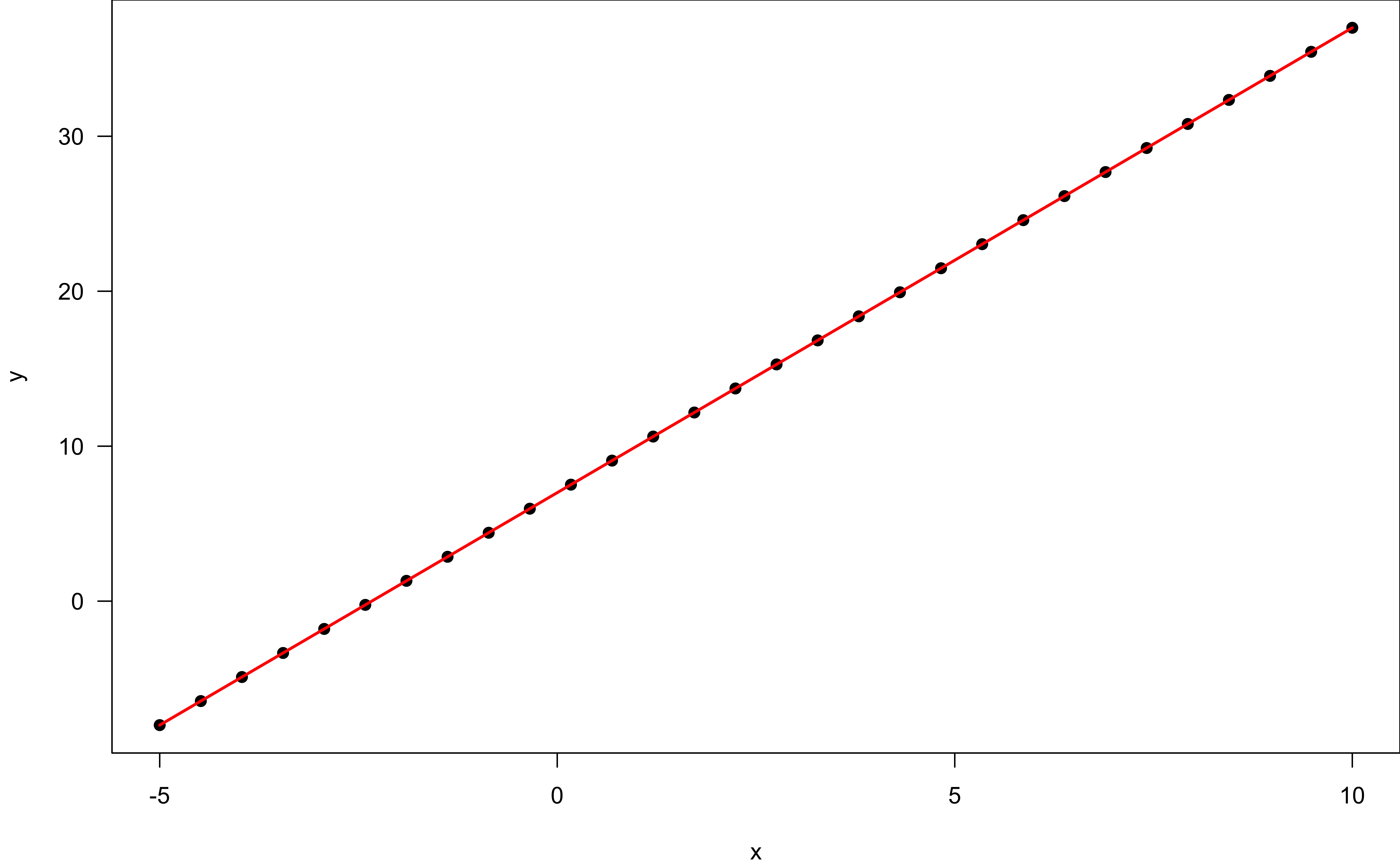
  • y = f(x) = 3x + 7 is a function with input x and output y.
  • If x = 5, y = 3 \times 5 + 7 = 22.

• In mathematics, how do we describe a Relationship Between Variables? We use a function. Right.
• The function y = f(x) gives us the relationship between an output Y and one or more inputs x.
  • You plug in the values of inputs and receive back the output value.
  • For example, the formula y = f(x) = 3x + 7 is a function with input x and output y. If x = 5, y = 3 \times 5 + 7 = 22.
• Because this is a linear function, we know that x and y are linearly related.
• With a value of x, I can give you 100% correct value of y, which is right on this straight line. right. In other words, their relationship is 100% deterministic.

Different Relationships

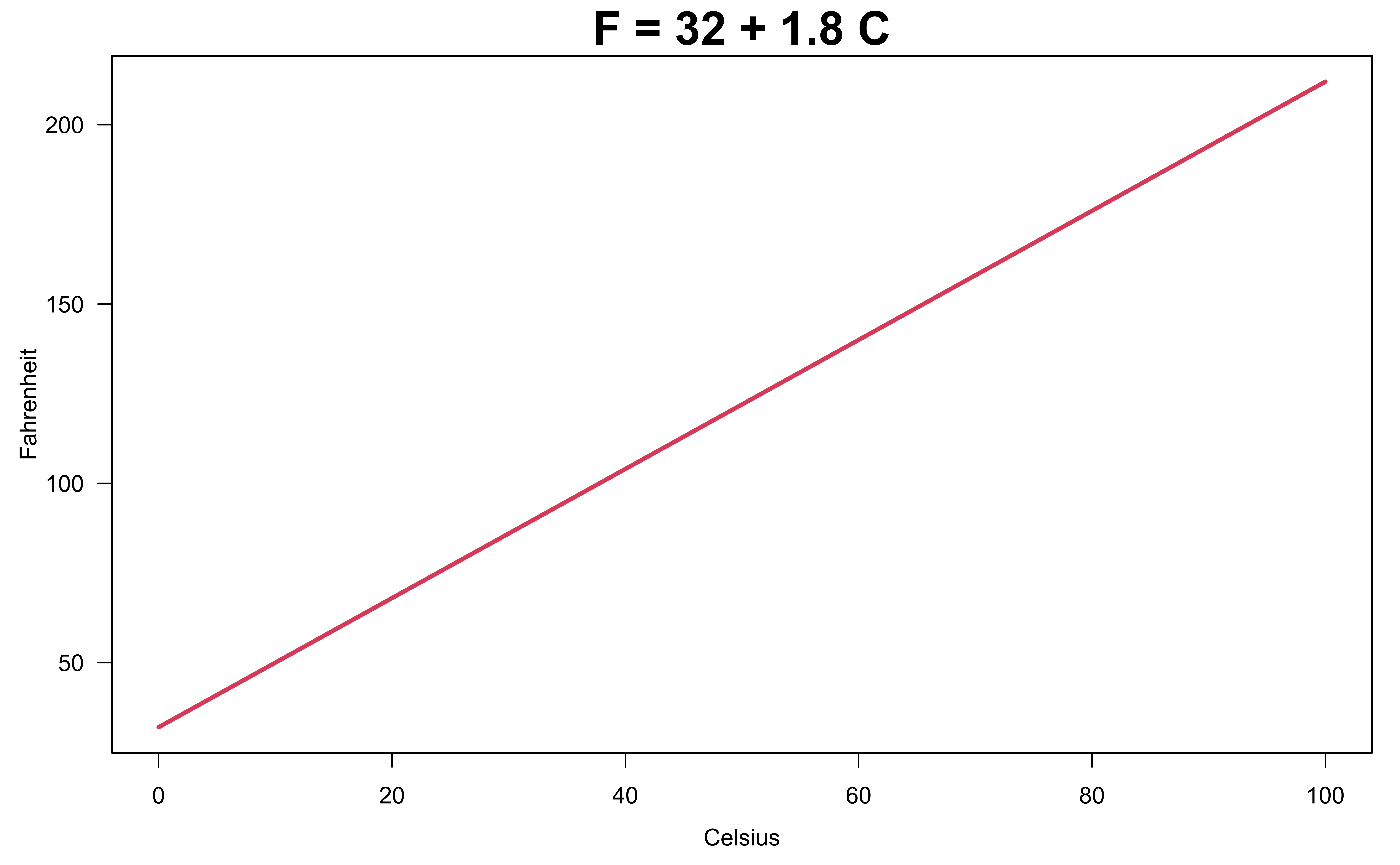
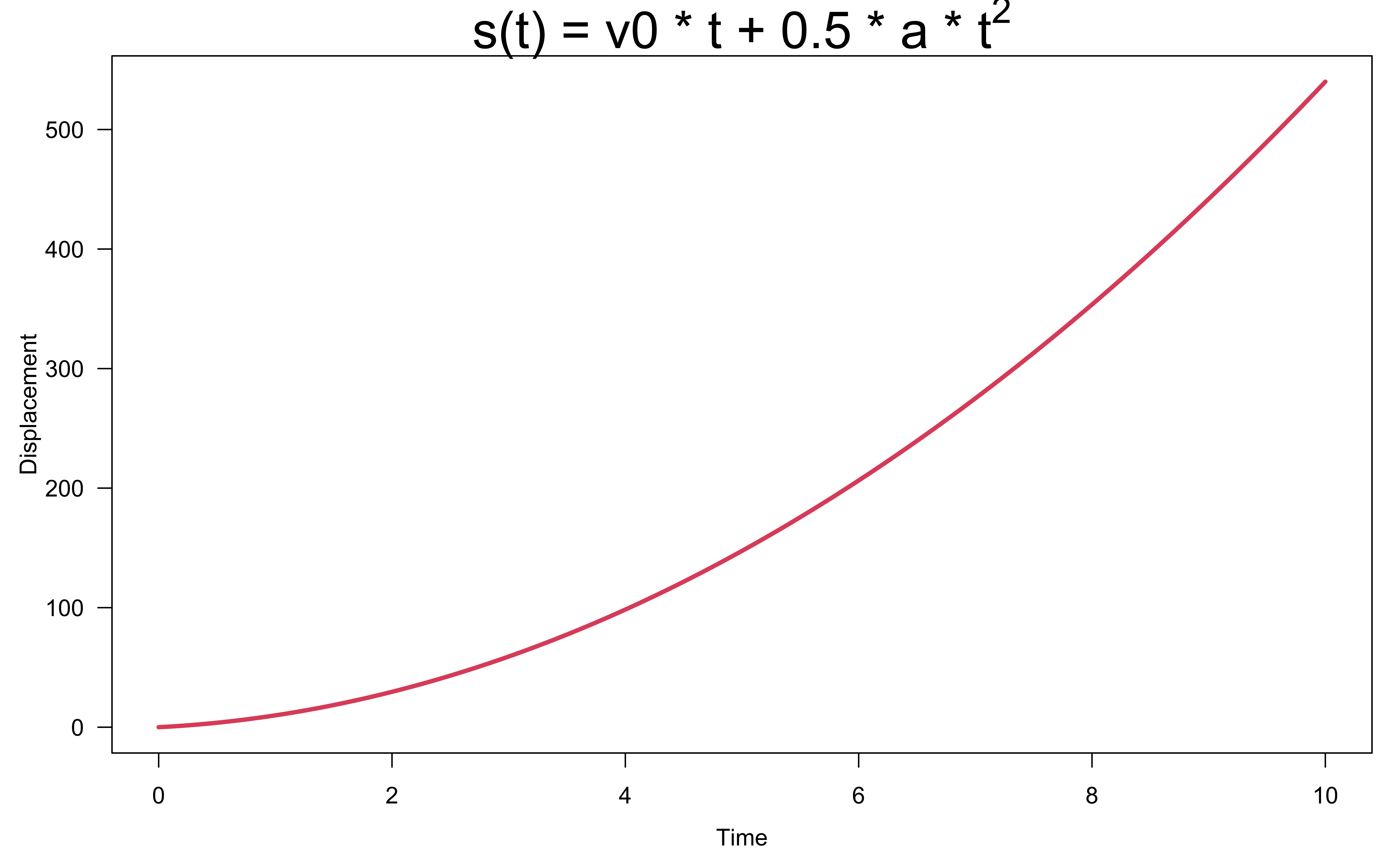
Can you come up with any real-world examples describing relationships between variables deterministically?

• The relationship between x and y can be more than linear.
• The relationship can be also quadratic, cubic or any other possible relationship.

Different Relationships

• Here I give your two examples. The first example is the conversion of F and C degrees. Their relationship is linear and F = 32 + 1.8 C.
• So you give me a C degree, I can tell you its corresponding F degree fro sure. Right.
• The second example comes from physics. the displacement of an object is a quadratic function of time.
• So here s(t) = v0 * t + 0.5 * a * t^2. v0 is the initial velocity, and a is acceleration, and t is time.
• Again the relationship between displacement and time is 100% deterministic.
• A value of time corresponds to an unique value of displacement given v0 and a.

Relationship between Variables is Not Perfect

Can you provide some real examples that the variables are related each other, but not perfectly related?

Relationship between Variables is Not Perfect

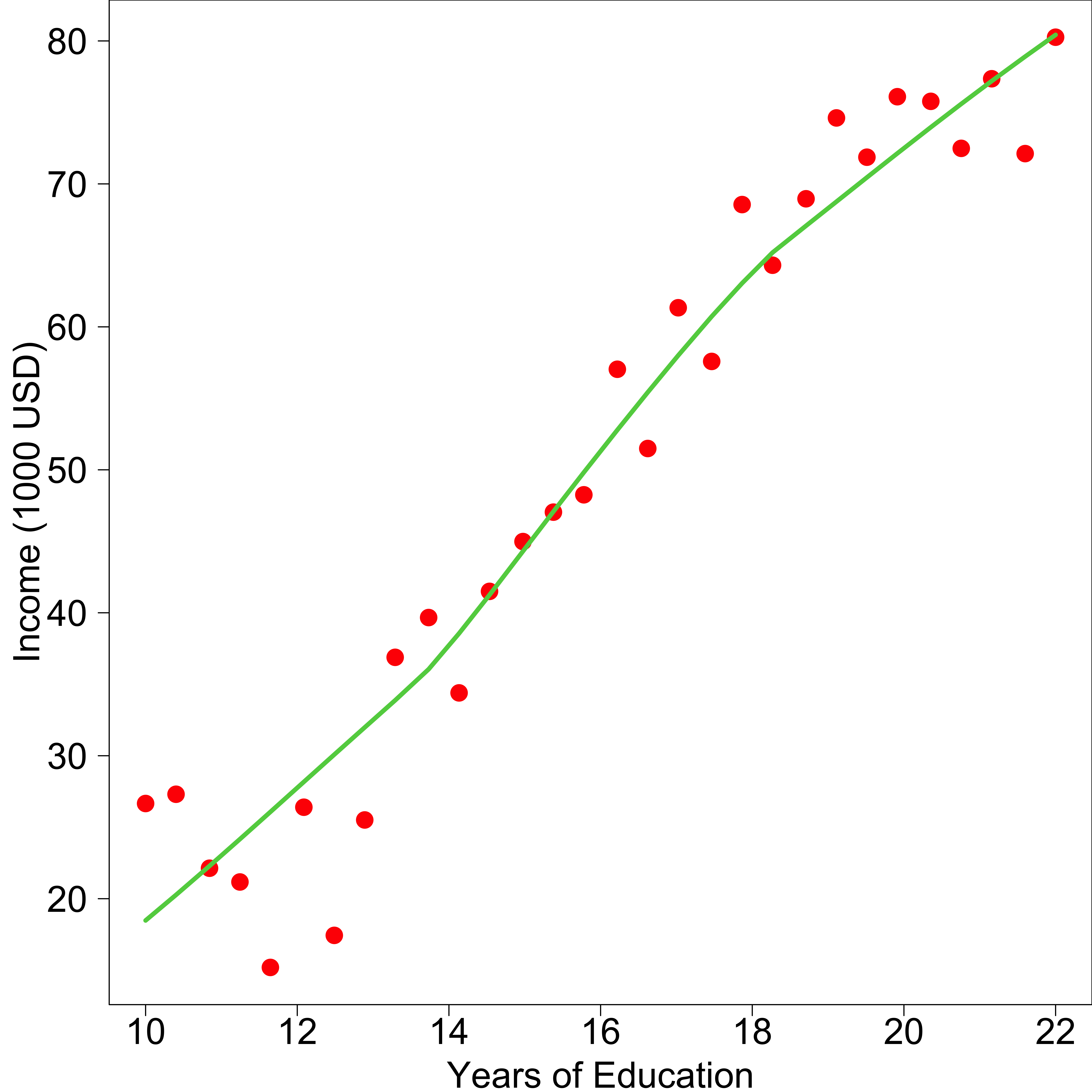
💵 In general, one with more years of education earns more.
💵 Any two with the same years of education may have different annual income.

• Here I give you a simple example: the relationship between income and years of education.
• 💵 In general, one with more years of education earns more.
• 💵 Any two with the same years of education may have different annual income.
• Because your income level depends on so many other factors, not just years of education.
• So when you plot the scatter plot of the two variables, you will find that there is some trend, but the data are sort of scattered or jittered or variated around some function that describes the relationship between income the years of education.
• Red dots are observed values or the years of education and income pairs.

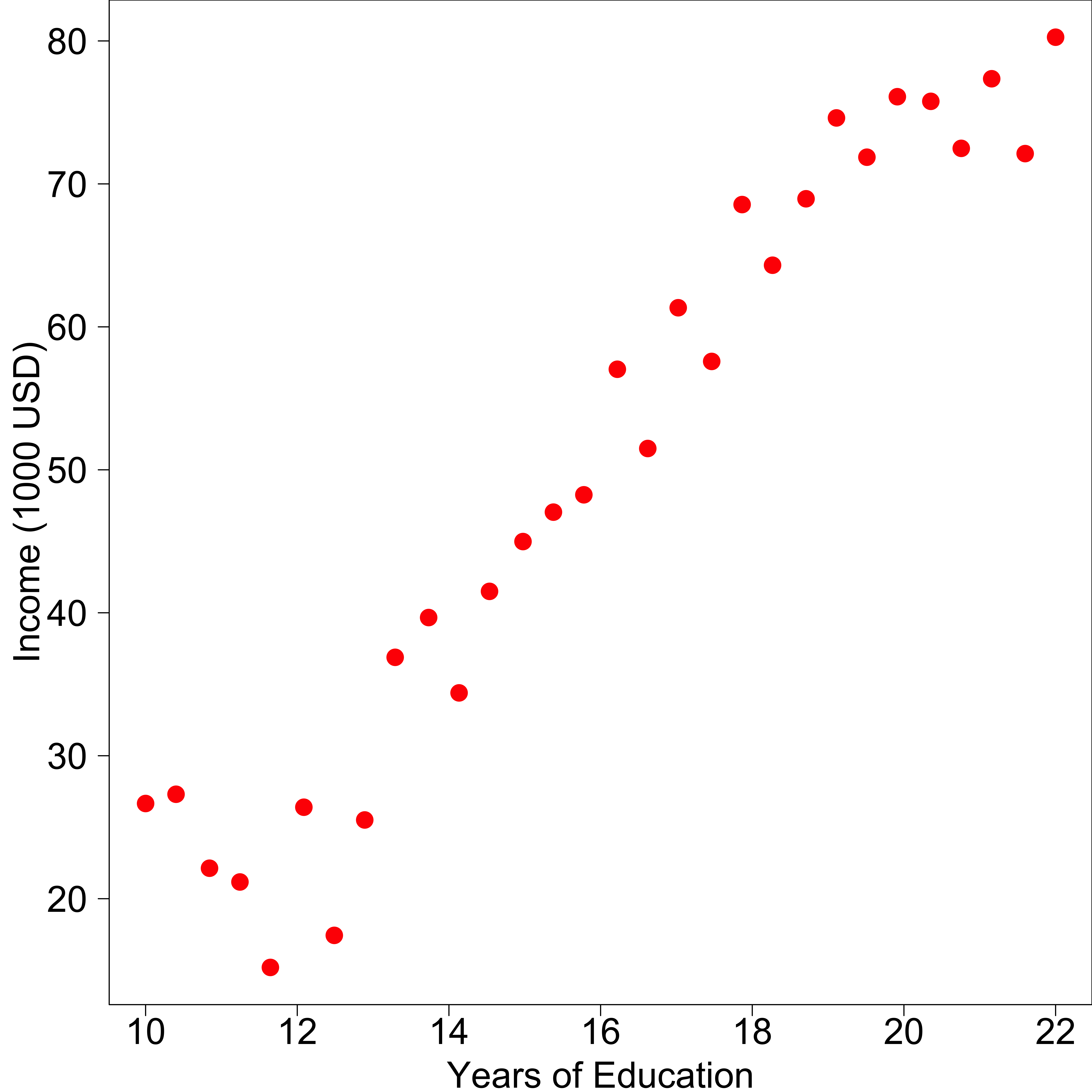
Variation around the Function/Model

What are the unexplained variation coming from?

• Other factors accounting for parts of variability of income.
  • Adding more explanatory variables to a model can reduce the variation size around the model.
• Pure measurement error.
• Just that randomness plays a big role. 🤔

What other factors (variables) may affect a person’s income?

your income = f(years of education, major, GPA, college, parent's income, ...)

• And the data Variation around the Function, or in general the regression model is just as important as the model, if not more!
  
• Basically, what statistics does is explain variation in the context of what remains unexplained.
• The scatter plot suggests that there might be other factors that account for large parts of variability.
• If that is the case, adding more explanatory variables ( Xs ) to a model can sometimes usefully reduce the size of the scatter around the model.
• Perhaps just that randomness plays a big role.

Supervised Learning Mapping

• Explain the relationship between X and Y and make predictions through a model Y = f(X) + \epsilon
• \epsilon: irreducible random error (Aleatoric Uncertainty)
  • independent of X
  • mean zero with some variance.
• f(\cdot): unknown function¹ describing the relationship between X and the mean of Y.

In Intro Stats, what is the form of f and what assumptions you made on the random error \epsilon ?

• f(X) = \beta_0 + \beta_1X with unknown parameters \beta_0 and \beta_1.
• \epsilon \sim N(0, \sigma^2).

• OK. Now after collecting the data of the variables we are interested, we know their relationship, most of the time, is not perfect, and stochastic in some way and in some sense.
• And how do we model such stochastic relationship? Well the answer is a regression model.
• Suppose we are interested in the relationship between two variables, call X and Y. In particular, we like to know how changes of X affect value of Y, or we want to use X to predict Y.
• In this sense, Y is called response, outcome, label, dependent variable, e.g., income
• X is called predictor, covariate, feature, regressor, explanatory or independent variable, e.g., years of education, which is known and fixed.
• Explain the relationship between X and Y and make predictions through a model Y = f(X) + \epsilon. This is a very general regression model we can built to learn the relationship b/w x and y.
• f(\cdot) is fixed but unknown and describes the true relationship between X and Y.
• \epsilon is a irreducible random error which is assumed to be independent of X and has mean zero with some variance.
• \epsilon is used to represent those measurement errors or the variation that cannot be explained or captured by the predictor X.
• Intro Stats:
  • f(X) = \beta_0 + \beta_1X with unknown parameters \beta_0 and \beta_1.
  • \epsilon \sim N(0, \sigma^2).
• X and Y are assumed to be linearly related, which may not be correct.
• Next week, we will learn simple linear regression from the scratch and in much more detail. Here I just give you an overview.

1. f(\cdot) is assumed fixed from frequentist point of view; f(\cdot) is random in the Bayesian framework.

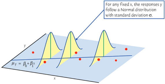
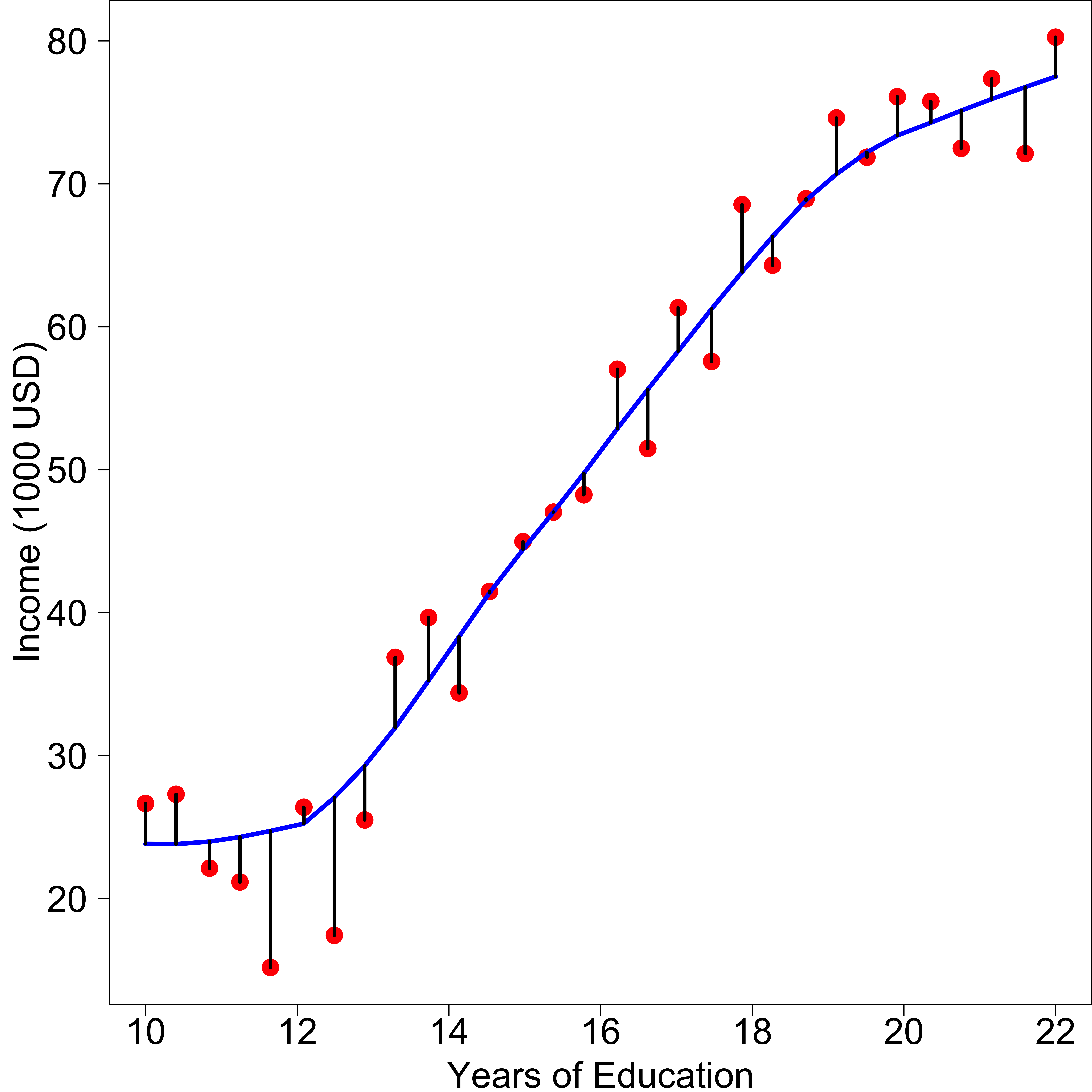
True Unknown Function f of the Model Y = f(X) + \epsilon

• Blue curve: true underlying relationship between (the mean) income and years of education.
• Black lines: error associated with each observation

Big problem: f(x) is unknown and needs to be estimated.

• Let’s go back to the income-education example. Red dots are observed values or the years of education and income pairs. Suppose we like to use a regression model y = f(x) + \epsilon to describe the relationship between income and education.
• And the *Blue** curve on the right shows the true underlying relationship between income and years of education, which is the function f in our regression model.
• And each Black vertical line indicates an error associated with each observation.
• So again, each red dot or observation is the value of the function f(x) plus some random error with its magnitude shown in a black vertical line.
• Again, in regression, we assume years of education is fixed. It is income level that varies around the function f.

How to Estimate f?

• Use training data \mathcal{D} = \{ (x_i, y_i) \}_{i=1}^n to train or teach our model to learn f.
• Use test data \mathcal{D}_{test} = \{ (x_j, y_j) \}_{j=1}^m to test or evaluate how well the model makes inference or prediction.

• Models are either parametric or nonparametric.

• Parametric methods involve a two-step model-based approach:
  • 1️⃣ Make an assumption about the shape of f, e.g. linear regression f(X) = \beta_0 + \beta_1X_1 + \beta_2X_2 + \dots + \beta_pX_p
  • 2️⃣ Use \mathcal{D} to train the model, e.g., learn the parameters \beta_j, j = 0, \dots, p using least squares.

• Nonparametric methods do not make assumptions about the shape of f.
  • Seek an estimate of f that gets close to the data points without being too rough or wiggly.

Parametric vs. Nonparametric Models

Parametric (Linear regression)

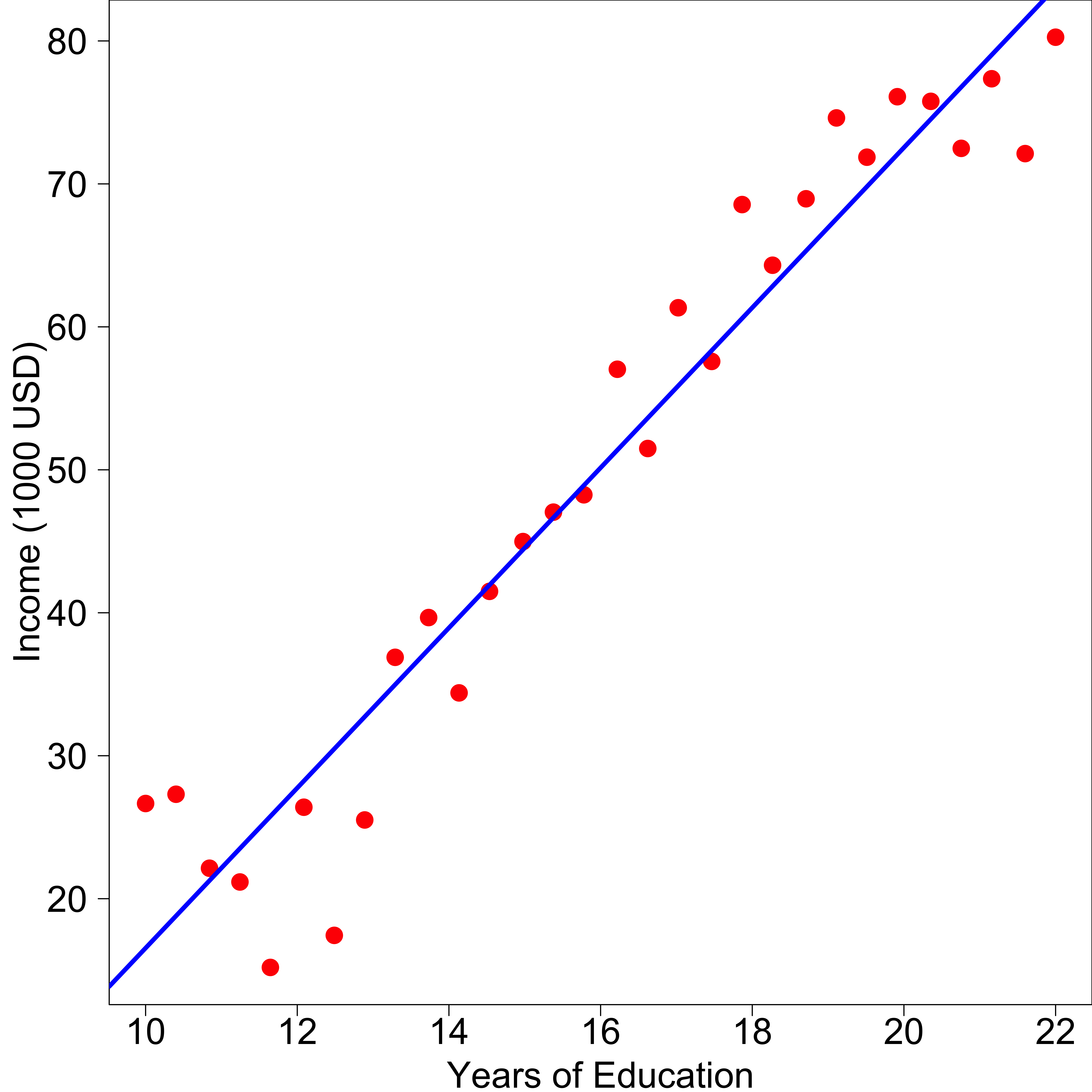
Nonparametric (LOESS)

Model Accuracy

No Free Lunch

• There is no free lunch in machine learning: no one method dominates all others over all possible data sets.

All models are wrong, but some are useful. – George Box (1919-2013)

• For any given training data, decide which method produces the best results.

• Selecting the best approach is one of the most challenging parts of machine learning.

• Need some way to measure how well its predictions actually match the training/test data.

• Numeric y: mean square error (MSE) for y with \hat{f} the estimated function of f \text{MSE}_{\texttt{Tr}} = \frac{1}{n} \sum_{i=1}^n (y_i - \hat{f}(x_i))^2, \quad \quad \text{MSE}_{\texttt{Te}} = \frac{1}{m} \sum_{j=1}^m (y_j - \hat{f}(x_j))^2

Are \text{MSE}_{\texttt{Tr}} and \text{MSE}_{\texttt{Te}} the same? When to use which?

Mean Square Error

• \text{MSE}_{\texttt{Tr}} measures how much \hat{f}(x_i) is close to the training data y_i (goodness of fit). However, most of the time

• We do not care how well the method works on the training data.

• We are interested in the predictive accuracy when we apply our method to previously unseen test data.

• We want to know whether \hat{f}(x_j) is (approximately) equal to y_j, where (x_j, y_j) is previously unseen or a test data point not used in training our model.

\text{MSE}_{\texttt{Tr}} or \text{MSE}_{\texttt{Te}} is smaller?

• \text{MSE}_{\texttt{Tr}} < \text{MSE}_{\texttt{Te}}.

• Most statistical learning methods either directly or indirectly seek to minimize the training MSE.
• Training data are the information we have and probably only have. Without other constraints or information about how we train the model, we tend to make use of all possible information in the training data to train our model.
• We want to know whether \hat{f}(x_j) is (approximately) equal to y_j, where (x_j, y_j) is a previously unseen test observation not used to train the model.

Model Complexity/Flexibility

• A more complex model produces a more flexible or wiggly regression curve \hat{f}(x) that matches the training data better.

• y = \beta_0+ \beta_1x + \beta_2x^2 + \cdots + \beta_{10}x^{10} + \epsilon is more complex than y = \beta_0+ \beta_1x + \epsilon

Overfitting: A too complex model fits the training data extremely well and too hard, picking up some patterns and variations simply caused by random noises that are not the properties of the true f, and not existed in the any unseen test data.

Underfitting: A model that is too simple to capture complex patterns or shapes of the true f(x). The estimate \hat{f}(x) is rigid and far away from data.

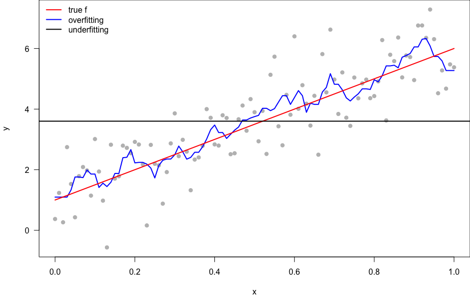
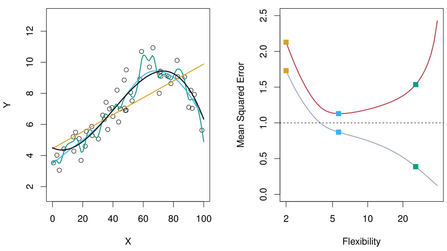
How \text{MSE}_{\texttt{Tr}} and \text{MSE}_{\texttt{Te}} change with model complexity?

Model Complexity/Flexibility and MSE

It’s common that no test data are available. Can we select a model that minimize \text{MSE}_{\texttt{Tr}}, since the training data and test data appear to be closed related?

• \text{MSE}_{\texttt{Tr}} (gray) is decreasing with the complexity.
• \text{MSE}_{\texttt{Te}} (red) is U-shaped: goes down then up with the complexity.

MSE	Overfit	Underfit
Train	tiny	big
Test	big	big

• No! There is no guarantee that the method with the lowest \text{MSE}_{\texttt{Tr}} will also have the lowest \text{MSE}_{\texttt{Te}}.

Bias-Variance Tradeoff

Given any new input x_0,

\text{MSE}_{\hat{f}} = E\left[\left(\hat{f}(x_0) - f(x_0)\right)^2\right] = \left[\text{Bias}\left(\hat{f}(x_0) \right)\right]^2 + \text{Var}\left(\hat{f}(x_0)\right)

where \text{Bias}\left(\hat{f}(x_0) \right) = E\left[ \hat{f}(x_0)\right] - f(x_0).

The expected test MSE of y_0 at x_0 is \text{MSE}_{y_0} = E\left[\left(y_0 - \hat{f}(x_0)\right)^2\right] = \text{MSE}_{\hat{f}} + \text{Var}(\epsilon)

Note

We never know the true expected test MSE, and prefer the model with the smallest expected test MSE estimate.

• Overfitting: Low bias and High variance

• Underfitting: High bias and Low variance

• MSE can be decomposed into two effects/measures
• MSE is a combination of two performance measures.

• Underfitting: On average, the estimate is far way from the truth. All estimates are close to each other.
• Overfitting: On average, the estimate is close to the truth. But estimates are far away from each other, leading to unstable and imprecise result.
• What we want is an estimate that balance the bias and variance, having the smallest test MSE.

Because bias and variance size change with model complexity or flexibility, choosing a model that balances bias and variance, or leads to the smallest MSE, is equivalent to choosing a model with just right complexity.

Lab: Bias-Variance Tradeoff

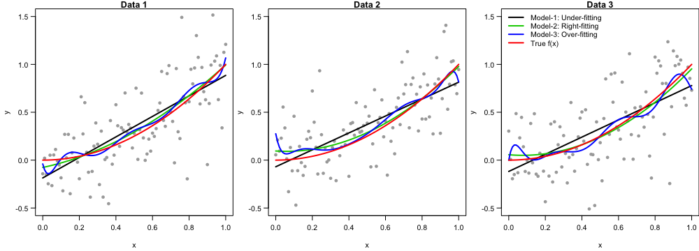
• Model 1: Under-fitting y = \beta_0+\beta_1x+\epsilon

• Model 2: Right-fitting y = \beta_0+\beta_1x+ \beta_2x^2 + \epsilon

• Model 3: Over-fitting y = \beta_0+\beta_1x+ \beta_2x^2 + \cdots + \beta_9x^9 + \epsilon

• To see expectation/bias and variance, we need replicates of training data.

Mean test error rate