Splines and General Additive Models 〰️
MSSC 6250 Statistical Machine Learning
Department of Mathematical and Statistical Sciences
Marquette University
Nonlinear Relationships
When \(y\) and \(x\) are Not Linearly Associated
Linear models can describe non-linear relationship.
Feature engineering: When \(y\) and \(x\) are not linearly associated, we transform \(x\) (sometimes also \(y\)) so that \(y\) and the transformed \(x\) become linearly related.
- Popular methods
- Basis function approach
- Local regression (MSSC 5780, ISL 7.6)
- Smoothing splines
- General additive models (GAMs)
Polynomial Regression
- The \(d\)th-order (degree) polynomial model in one variable is \[y = \beta_0 + \beta_1 x + \beta_2 x^2 + \cdots + \beta_dx^d + \epsilon\]
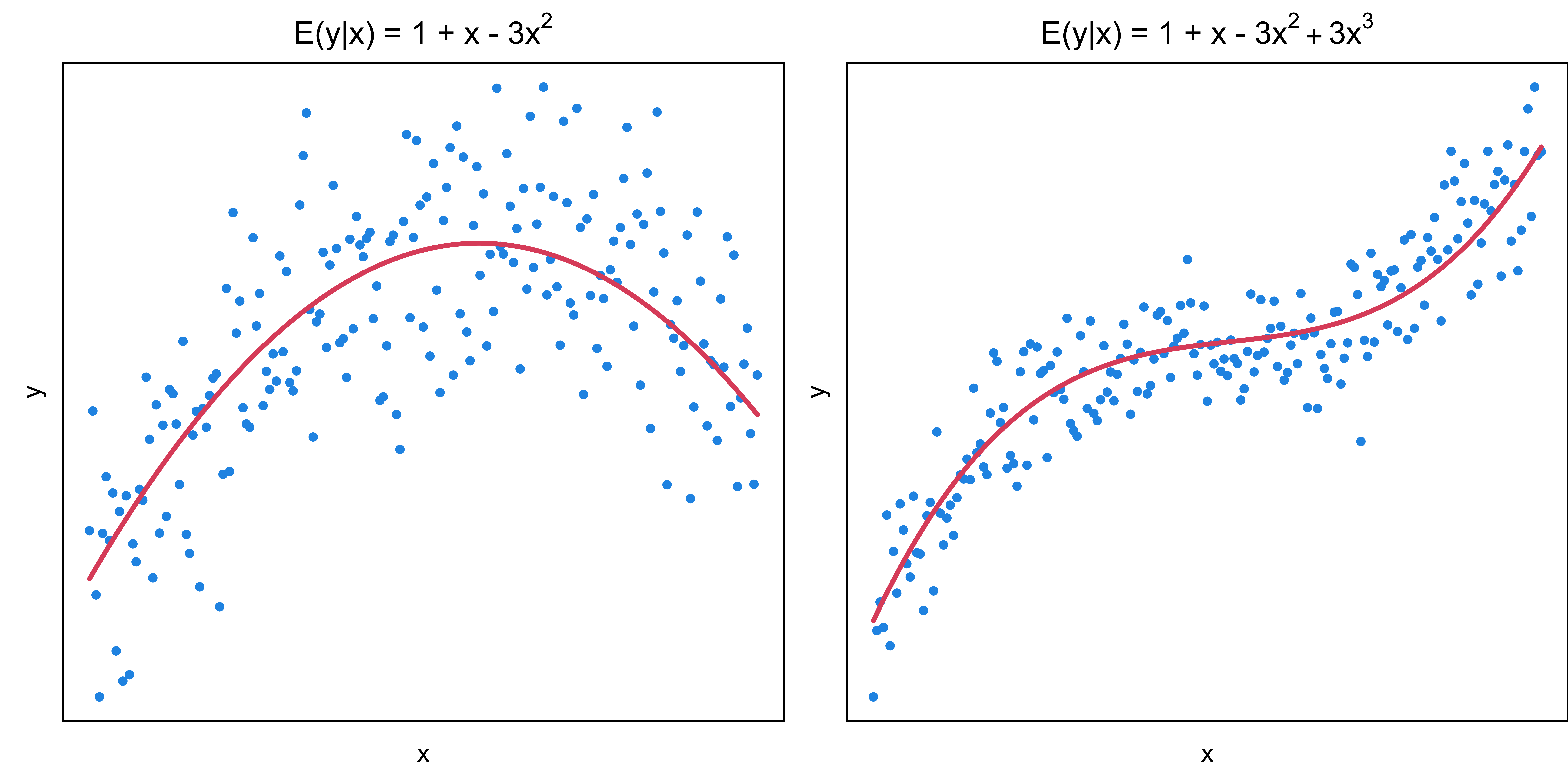
- We extend the simple linear regression by mapping \(x\) to \((x, x^2, \dots, x^d)\).
Basis Function Approach
- A set of basis functions or transformations that can be applied to a variable \(x\):\[[b_1(x), b_2(x), \dots , b_K(x)]\]
- (Adaptive) basis function model: \[y = \beta_0 + \beta_1 b_1(x) + \beta_2 b_2(x) + \cdots + \beta_K b_K(x) + \epsilon\]
Is polynomial regression a basis function approach?
- Polynomial basis: \(\phi(x) = [1, x, x^2, \dots, x^K]\)
- Fourier series basis: \(\phi(x) = [1, \cos(\omega_1x + \psi_1), \cos(\omega_2x + \psi_2), \dots]\)
- B-Spline basis
Important
\([b_1(x), b_2(x), \dots , b_K(x)]\) are fixed and known.
Piecewise regression
Polynomial regression imposes a global structure on the non-linear function.
Piecewise regression allows structural changes in different parts of the range of \(x\)
\[y=\begin{cases} \beta_{01} + \beta_{11}x+ \beta_{21}x^2 +\epsilon & \quad \text{if } x < \xi\\ \beta_{02} + \beta_{12}x+ \beta_{22}x^2+\beta_{32}x^3+\epsilon & \quad \text{if } x \ge \xi \end{cases}\]
The joint points of pieces are called knots.
Using more knots leads to a more flexible piecewise polynomial.
With \(K\) different knots, how many different polynomials do we have?
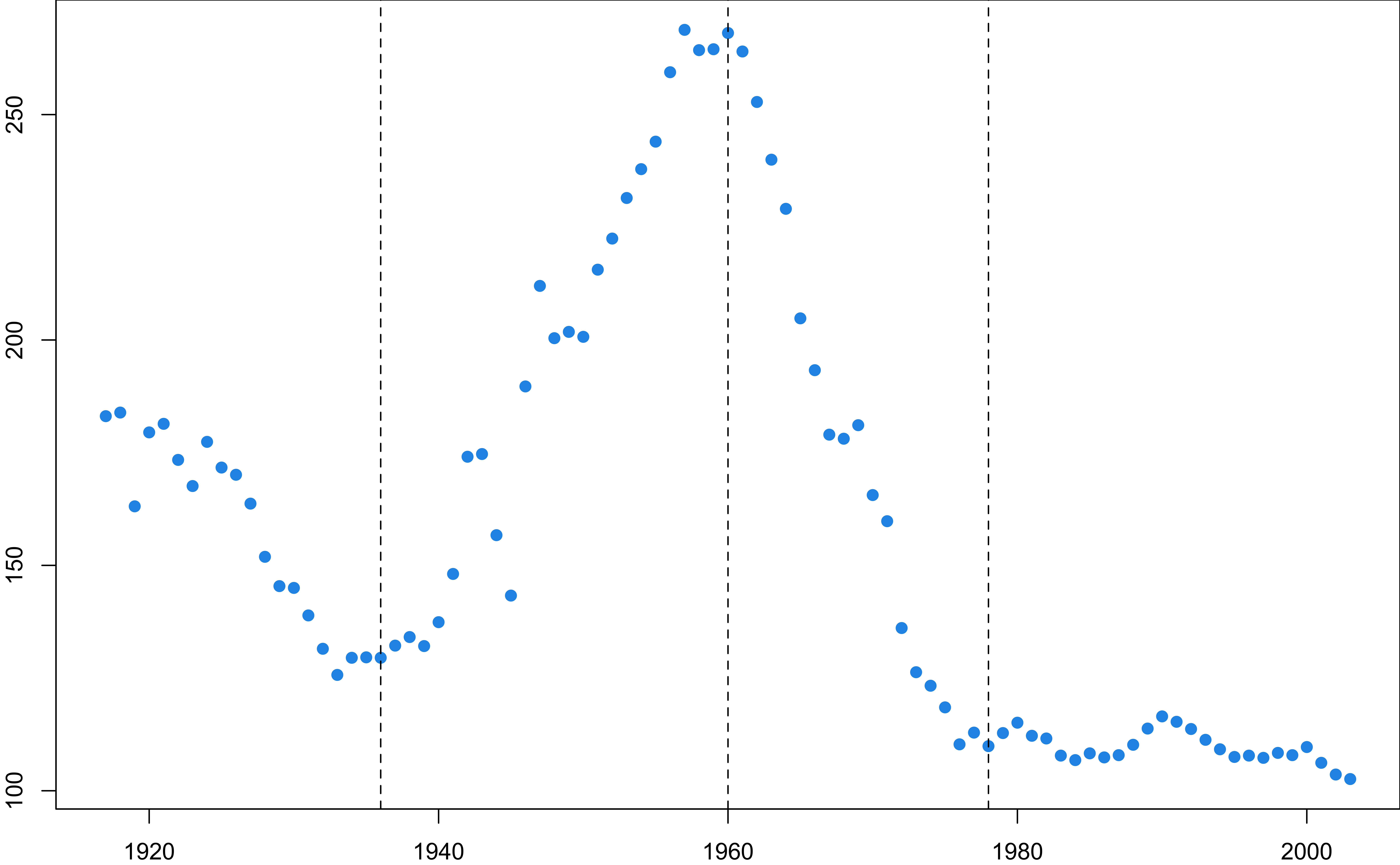
U.S. Birth Rate from 1917 to 20031
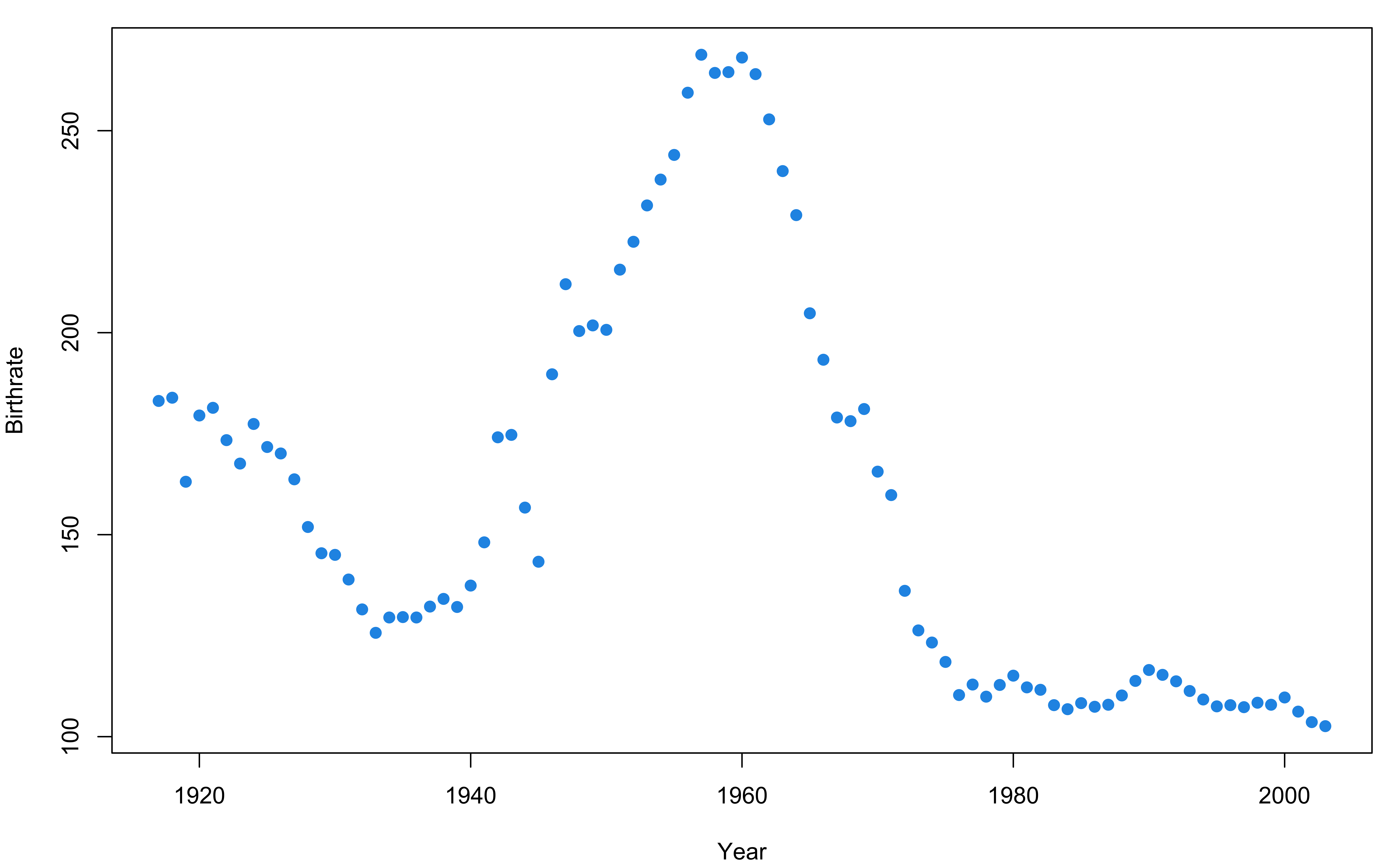
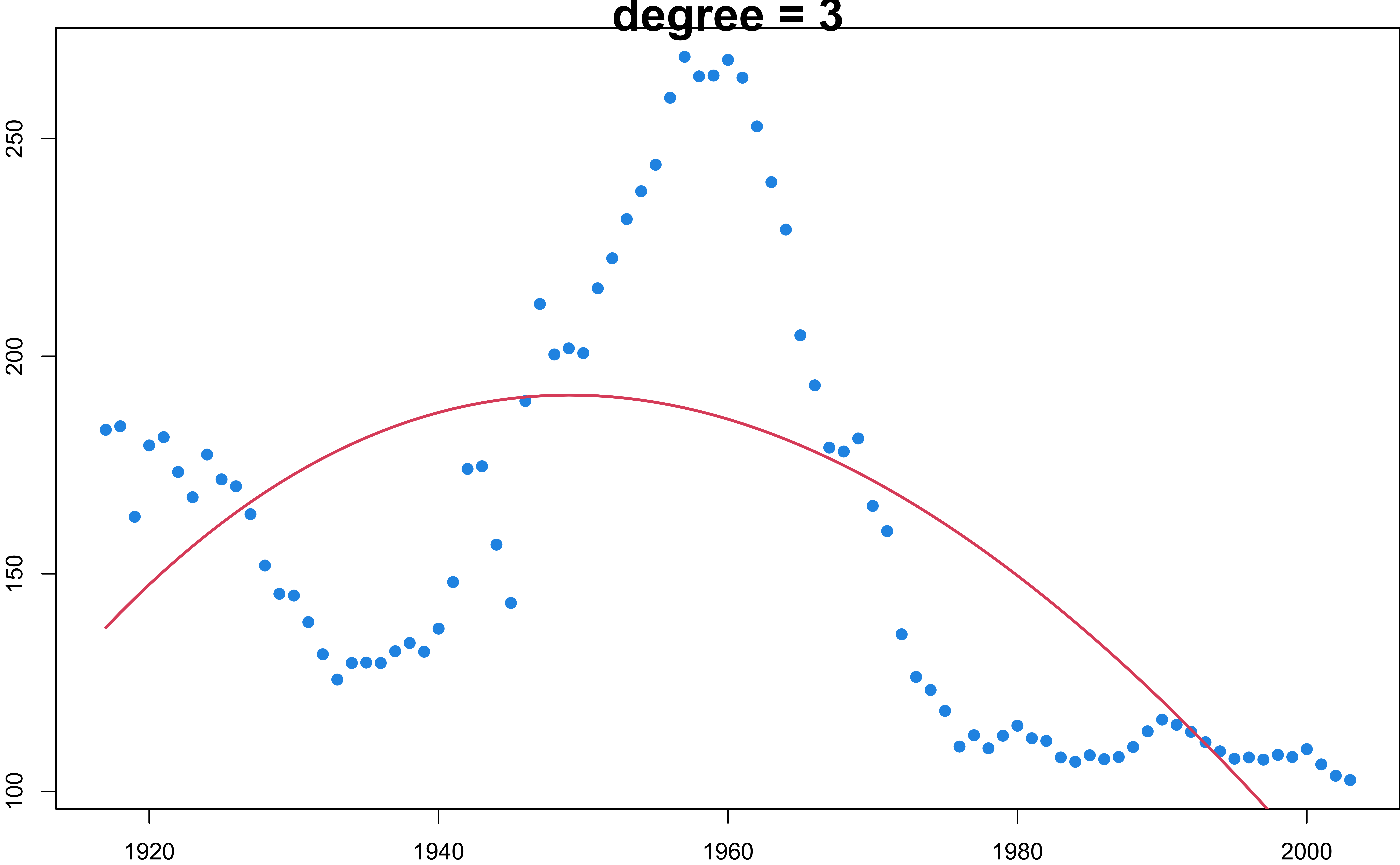
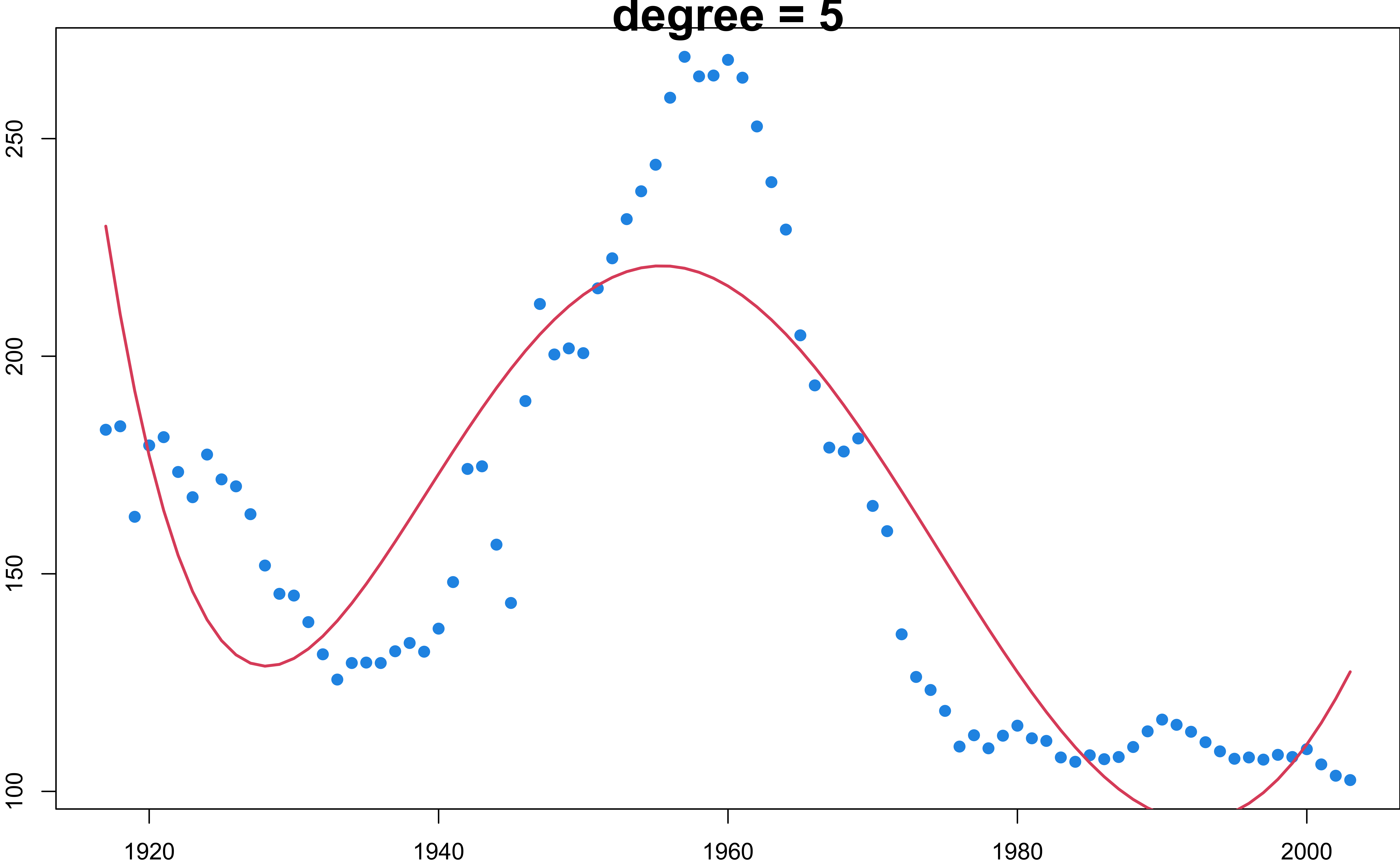
A Polynomial Regression Provide a Poor Fit
Piecewise Polynomials: 3 knots at 1936, 60, 78
\[y=\begin{cases} \beta_{01} + \beta_{11}x+ \epsilon & \text{if } x < 1936\\ \beta_{02} + \beta_{12}x+\epsilon & \text{if } 1936 \le x < 1960 \\ \beta_{03} + \beta_{13}x+\epsilon & \text{if } 1960 \le x < 1978 \\ \beta_{04} + \beta_{14}x+\epsilon & \text{if } 1978 \le x \end{cases}\]
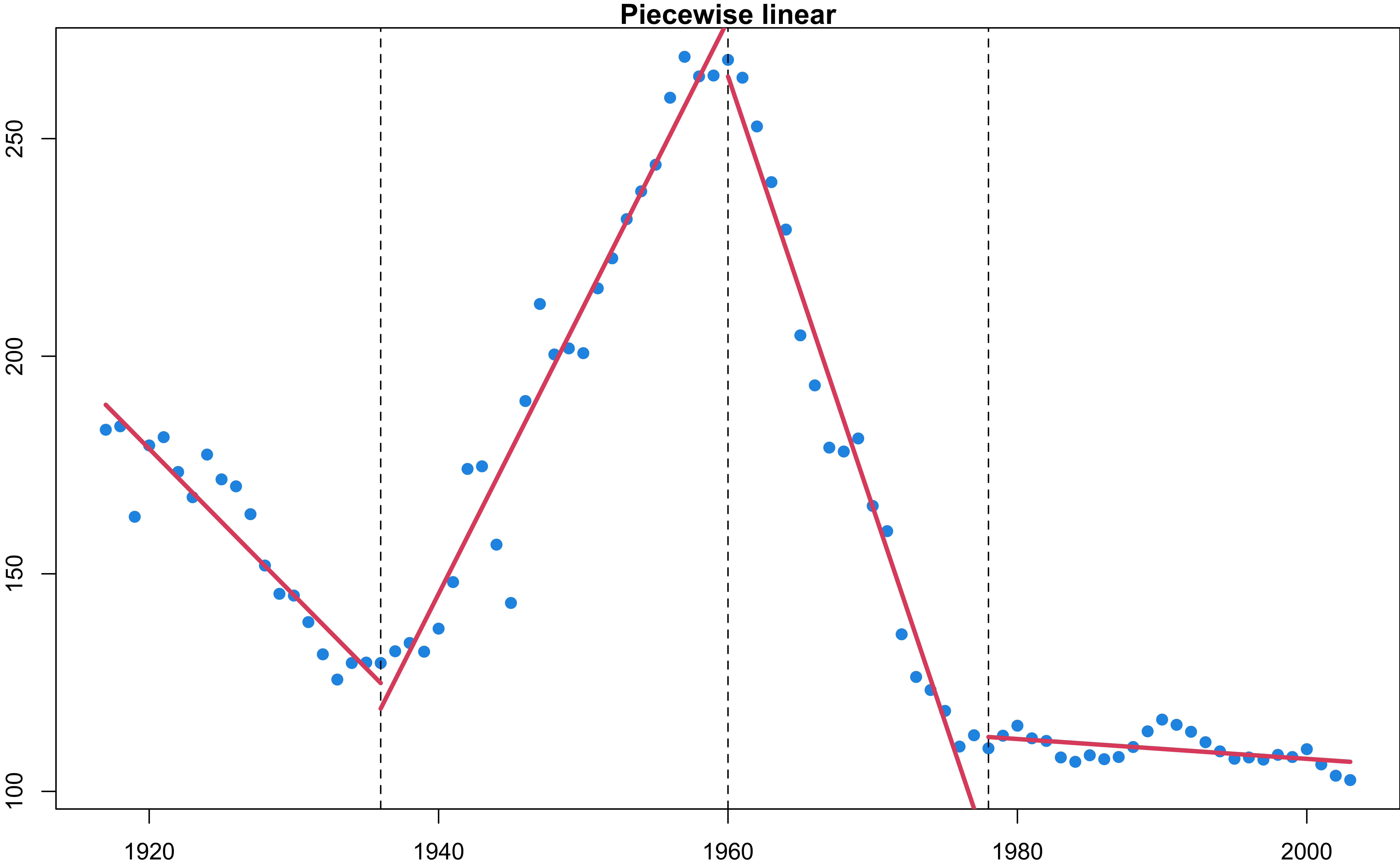
Any issue of piecewise polynomials?
Regression Splines
Piecewise polynomials + Continuity/Differentiability at knots
Splines
Splines of degree \(d\) are smooth piecewise polynomials of degree \(d\) with continuity in derivatives (smoothing) up to degree \(d-1\) at each knot.
How do we turn the piecewise regression of degree 1 into a regression spline?
\[y=\begin{cases} \beta_{01} + \beta_{11}x+ \epsilon & \quad \text{if } x < 1936\\ \beta_{02} + \beta_{12}x+\epsilon & \quad \text{if } 1936 \le x < 1960 \\ \beta_{03} + \beta_{13}x+\epsilon & \quad \text{if } 1960 \le x < 1978 \\ \beta_{04} + \beta_{14}x+\epsilon & \quad \text{if } 1978 \le x \end{cases}\]
- For splines of degree 1, we require continuous piecewise linear function
\[\begin{align} \beta_{01} + \beta_{11}1936 &= \beta_{02} + \beta_{12}1936\\ \beta_{02} + \beta_{12}1960 &= \beta_{03} + \beta_{13}1960\\ \beta_{03} + \beta_{13}1978 &= \beta_{04} + \beta_{14}1978 \end{align}\]
splines::bs()
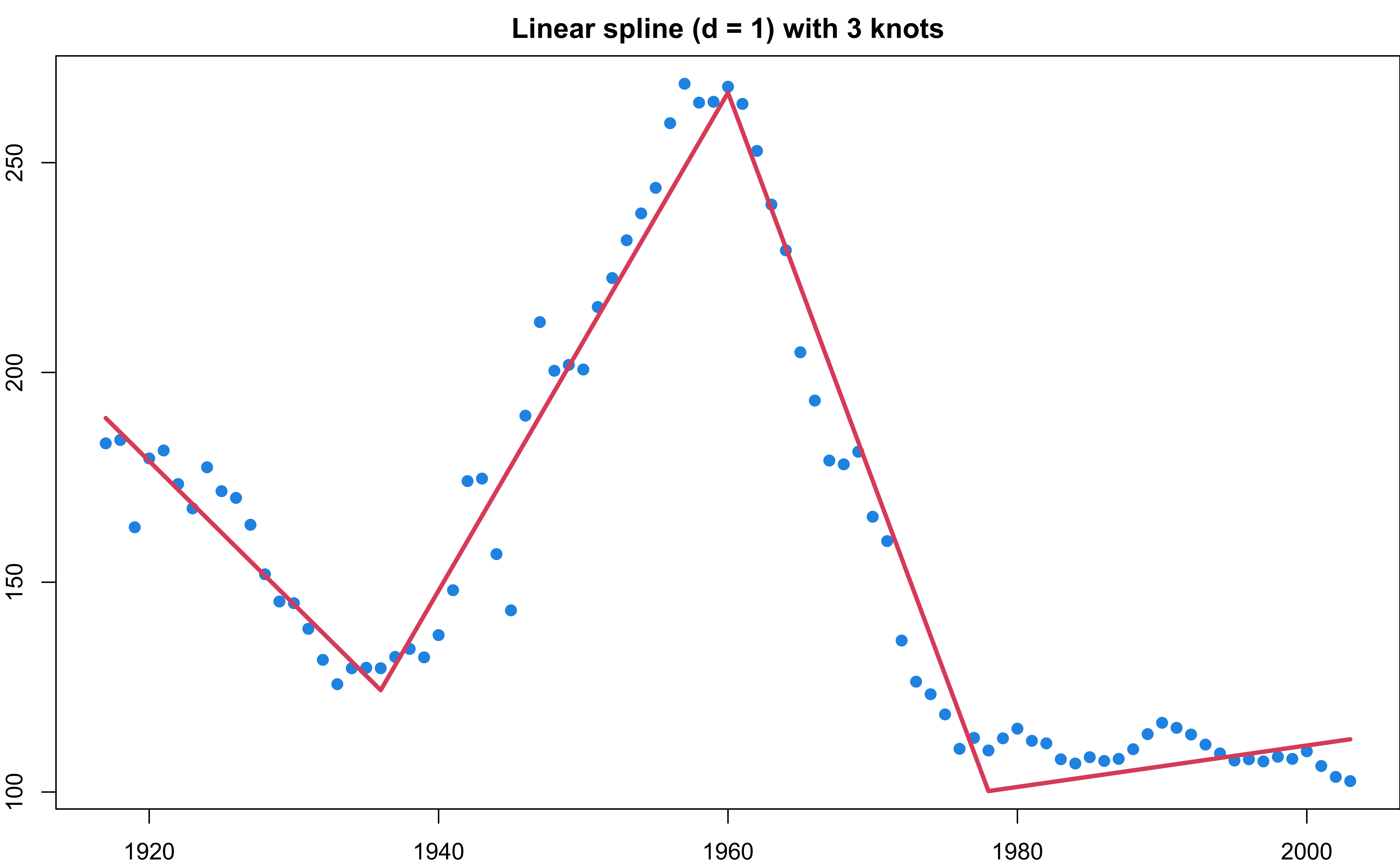
The function is continuous everywhere, also at knots \(\xi_1, \xi_2,\) and \(\xi_3\), i.e. \(f_{k}(\xi_k^-) = f_{k+1}(\xi_k^+)\).
Linear everywhere except \(\xi_1, \xi_2,\) and \(\xi_3\).
Has a different slope for each region.
Splines as Basis Function Model
For linear splines with 3 knots,
\[\begin{align} b_1(x) &= x\\ b_2(x) &= (x - \xi_1)_+\\ b_3(x) &= (x - \xi_2)_+\\ b_4(x) &= (x - \xi_3)_+ \end{align}\] where
- \((x - \xi_k)_+\) is a truncated power basis function (of power one) such that
\[(x - \xi_k)_+=\begin{cases} x - \xi_k & \quad \text{if }x > \xi_k\\ 0 & \quad \text{otherwise} \end{cases}\]
\[\begin{align} y &= \beta_0 + \beta_1 b_1(x) + \beta_2 b_2(x) + \beta_3 b_3(x) + \beta_4 b_4(x) + \epsilon\\ &=\beta_0 + \beta_1 x + \beta_2 (x - \xi_1)_+ + \beta_3 (x - \xi_2)_+ + \beta_4 (x - \xi_3)_+ + \epsilon \end{align}\]
Linear Splines Basis Functions
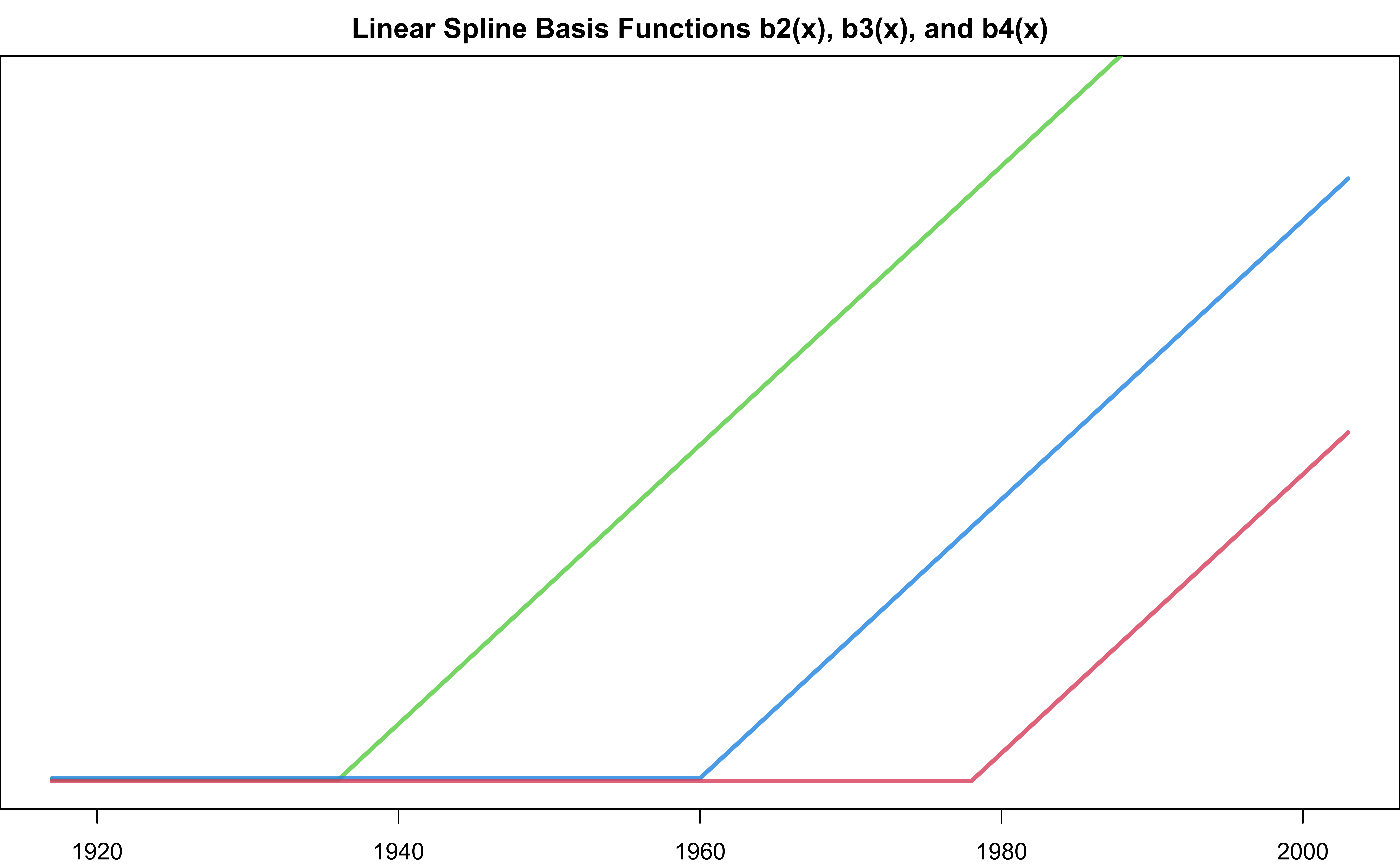
Splines as Basis Function Model1
With degree \(d\) and \(K\) knots, the regression spline with first \(d-1\) derivatives being continuous at the knots can be represented as
\[\begin{align} y &= \beta_0 + \beta_1 b_1(x) + \beta_2 b_2(x) + \dots + \beta_d b_d(x) + \beta_{d+1}b_{d+1}(x) + \dots + \beta_{d+K}b_{d+K}(x) + \epsilon \end{align}\] where
\(b_j(x) = x^j, j = 1, 2, \dots, d\)
\(b_{d+k} = (x - \xi_k)^{d}_+, k = 1, \dots, K\) where \[(x - \xi_k)^d_+=\begin{cases} (x - \xi_k)^d & \quad \text{if }x > \xi_k\\ 0 & \quad \text{otherwise} \end{cases}\]
Can you write the model with \(d = 2\) and \(K = 3\)?
Cubic Splines1
- The cubic spline is a spline of degree 3 with first 2 derivatives are continuous at the knots.
\[\begin{align} y &= \beta_0 + \beta_1 x + \beta_2 x^2 + \beta_3 x^3 + \sum_{k = 1}^K \beta_{k+3} (x - \xi_k)_+^3 + \epsilon \end{align}\]
- Smooth at knots because
- \(f(\xi_k^-) = f(\xi_k^+)\)
- \(f'(\xi_k^-) = f'(\xi_k^+)\)
- \(f''(\xi_k^-) = f''(\xi_k^+)\)
- But \(f^{(3)}(\xi_k^-) \ne f^{(3)}(\xi_k^+)\)
Degrees of Freedom
In regression, (effective) degrees of freedom (df) can be viewed as the number of regression coeffcients that are freely to move.
It measures the model complexity/flexiblity. The larger df is, the more flexible the model is.
- Piecewise linear: 3 knots, 4 linear regressions, and 8 dfs.
\[y=\begin{cases} \beta_{01} + \beta_{11}x+ \epsilon & \quad \text{if } x < 1936\\ \beta_{02} + \beta_{12}x+\epsilon & \quad \text{if } 1936 \le x < 1960 \\ \beta_{03} + \beta_{13}x+\epsilon & \quad \text{if } 1960 \le x < 1978 \\ \beta_{04} + \beta_{14}x+\epsilon & \quad \text{if } 1978 \le x \end{cases}\]
- Linear splines (continuous piecewise linear): 8 - 3 constraints = 5 dfs. (Check its basis representation)
\[\begin{align} \beta_{01} + \beta_{11}1936 &= \beta_{02} + \beta_{12}1936\\ \beta_{02} + \beta_{12}1960 &= \beta_{03} + \beta_{13}1960\\ \beta_{03} + \beta_{13}1978 &= \beta_{04} + \beta_{14}1978 \end{align}\]
Degrees of Freedom
- With degree \(d\) and \(K\) knots,
\[\text{df} = K + d + 1\]
So what is the degrees of freedom of cubic splines?
Cubic Splines
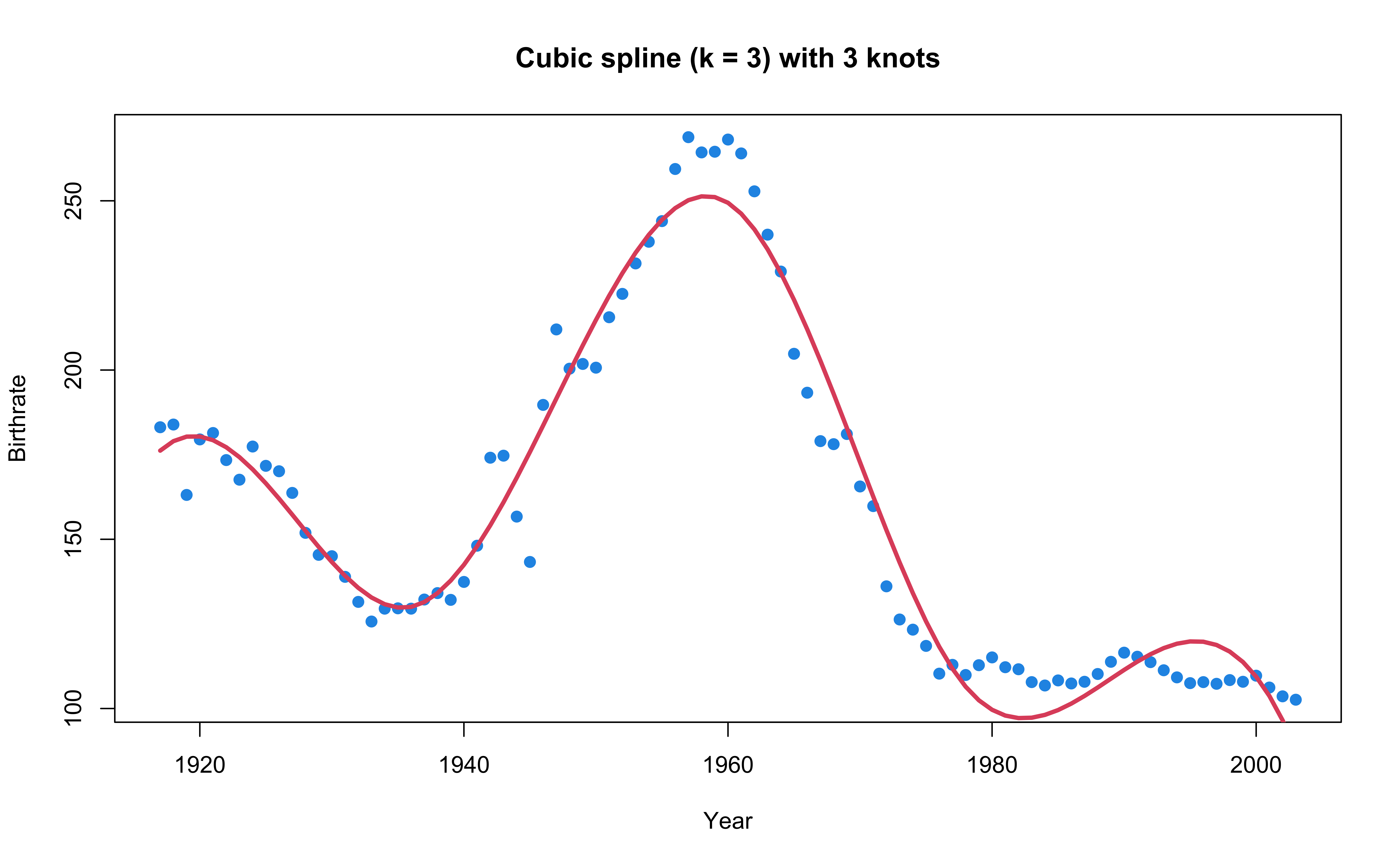
Natural Splines
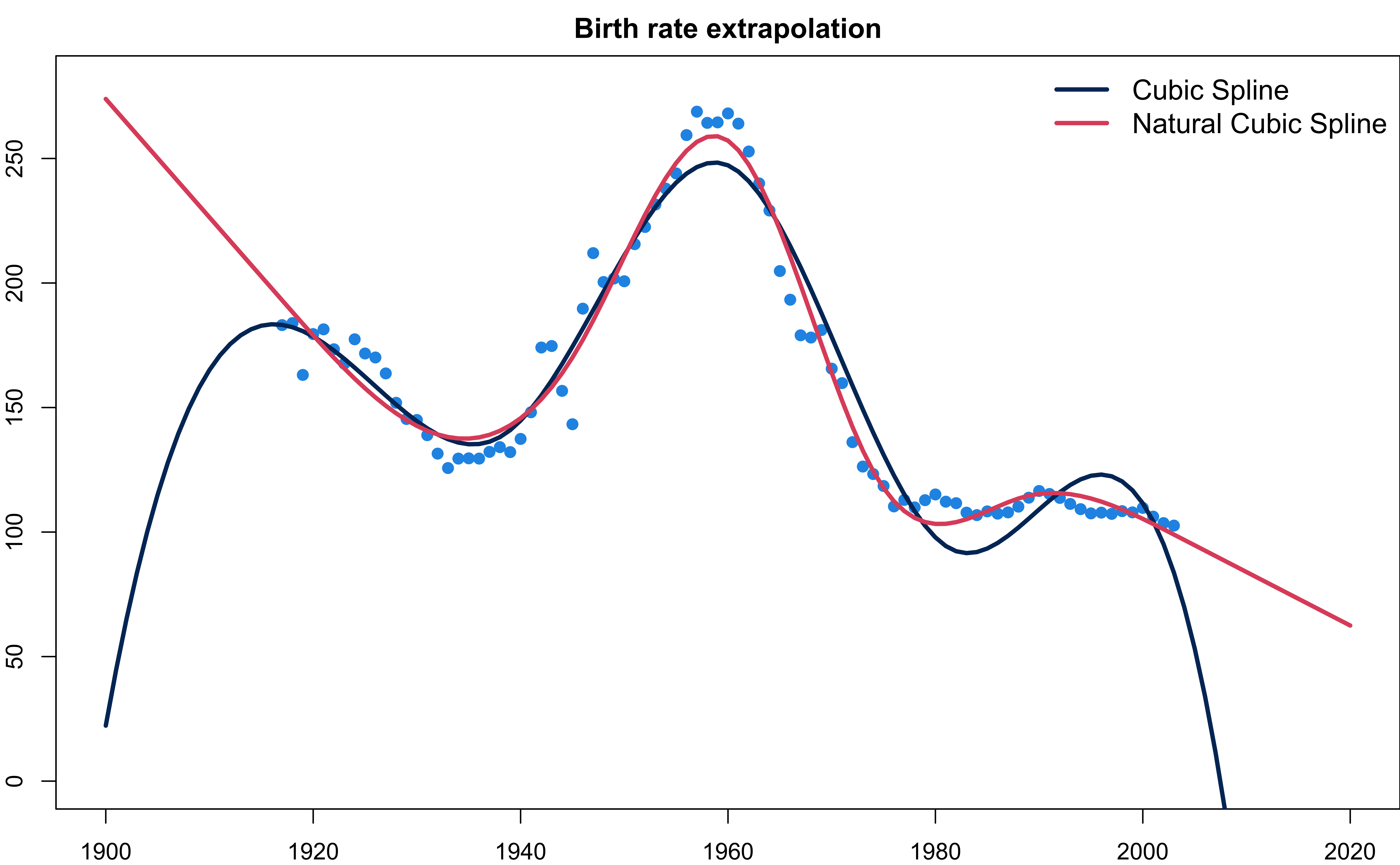
- Splines1 tends to produce erratic and undesirable results near the boundaries, and huge variance at the outer range of the predictors.
- A natural spline is a regression spline with additional boundary constraints:
- The spline function is linear at the boundary (in the region where \(X\) is smaller than the smallest knot, or larger than the largest knot).
Natural splines generally produce more stable estimates at the boundaries.
Assuming linearity near the boundary is reasonable since there is less information available there.
Natural Cubic Spline (NCS) forces the 2nd and 3rd derivatives to be zero at the boundaries.
The constraints frees up 4 dfs.
The df of NCS is \(K\).
Spline and Natural Spline Comparison
- Cubic Spline vs. Natural Cubic Spline with the same degrees of freedom 6.
Practical Issues
-
How many knots should we use
- As few knots as possible, with at least 5 data points per segment (Wold, 1974)
- Cross-validation: e.g., choose the \(K\) giving the smallest \(MSE_{CV}\)
-
Where to place the knots
- No more than one extreme or inflection point per segment (Wold, 1974)
- If possible, the extreme points should be centered in the segment
- More knots in places where the function might vary most rapidly, and fewer knots where it seems more stable
- Place knots in a uniform fashion
-
Specify the desired df, and have the software place the corresponding number of knots at uniform quantiles of the data (
bs(),ns())
-
Degree of functions in each region
- Use \(d < 4\) to avoid overly flexible curve fitting
- Cubic spline is popular
Smoothing Splines
Roughness Penalty Approach
Our goal is inference or curve fitting rather than out of range prediction or forecasting.
Is there a method that we can select the number and location of knots automatically?
Consider this criterion for fitting a smooth function \(g(x)\) to some data:
\[\begin{equation} \min_{g} \sum_{i=1}^n \left( y_i - g(x_i) \right)^2 + \lambda \int g''(t)^2 \, dt \end{equation}\]
The first term is \(SS_{res}\), and tries to make \(g(x)\) match the data at each \(x_i\). (Goodness-of-fit)
The second term with \(\lambda \ge 0\) is a roughness penalty and controls how wiggly \(g(x)\) is.
Loss + Penalty
Roughness Penalty Approach
\[\begin{equation} \min_{g} \sum_{i=1}^n \left( y_i - g(x_i) \right)^2 + \lambda \int g''(t)^2 \, dt \end{equation}\]
How \(\lambda\) affects the shape of \(g(x)\)?
The smaller \(\lambda\) is, the more wiggly \(g(x)\) is, eventually interpolating \(y_i\) when \(\lambda = 0\).
As \(\lambda \rightarrow \infty\), \(g(x)\) becomes linear.
The function \(g\) that minimizes the objective is known as a smoothing spline.
Note
- The solution \(\hat{g}\) is a natural cubic spline, with knots at \(x_1, x_2, \dots , x_n\)!
- But, it is not the same NCS gotten from the basis function approach.
- It is a shrunken version where \(\lambda\) controls the level of shrinkage.
- Its effective df is less than \(n\).
Properties of Smoothing splines
- Smoothing splines avoid the knot-selection issue, leaving a single \(\lambda\) to be chosen.
Linear regression
\(\hat{\mathbf{y}} = \bf H \mathbf{y}\) where \(\bf H\) is the hat matrix
The degrees of freedom \((\text{# coef})\) is \[p = \sum_{i=1}^n {\bf H}_{ii}\]
PRESS for model selection
\[\begin{align} PRESS &= \sum_{i = 1}^n \left( y_i - \hat{y}_i^{(-i)}\right)^2 \\ &= \sum_{i = 1}^n \left[ \frac{y_i - \hat{y}_i}{1 - {\bf H}_{ii}}\right]^2\end{align}\]
Smoothing splines
\(\hat{\mathbf{g}}_{\lambda} = {\bf S}_{\lambda} \mathbf{y}\) where \(\bf {\bf S}_{\lambda}\) is the smoother matrix.
The effective degrees of freedom \((\text{# coef})\) is \[df_{\lambda} = \sum_{i=1}^n \{{\bf S}_{\lambda}\}_{ii} \in [2, n]\]
LOOCV for choosing \(\lambda\)1
\[\begin{align} (SS_{res})_{CV}(\lambda) &= \sum_{i = 1}^n \left( y_i - \hat{g}_{\lambda}^{(-i)}(x_i)\right)^2 \\ &= \sum_{i = 1}^n \left[ \frac{y_i - \hat{g}_{\lambda}(x_i)}{1 - \{{\bf S}_{\lambda}\}_{ii}}\right]^2 \end{align}\]
smooth.spline()
-
cv = TRUEuse LOOCV;cv = FALSEuse GCV
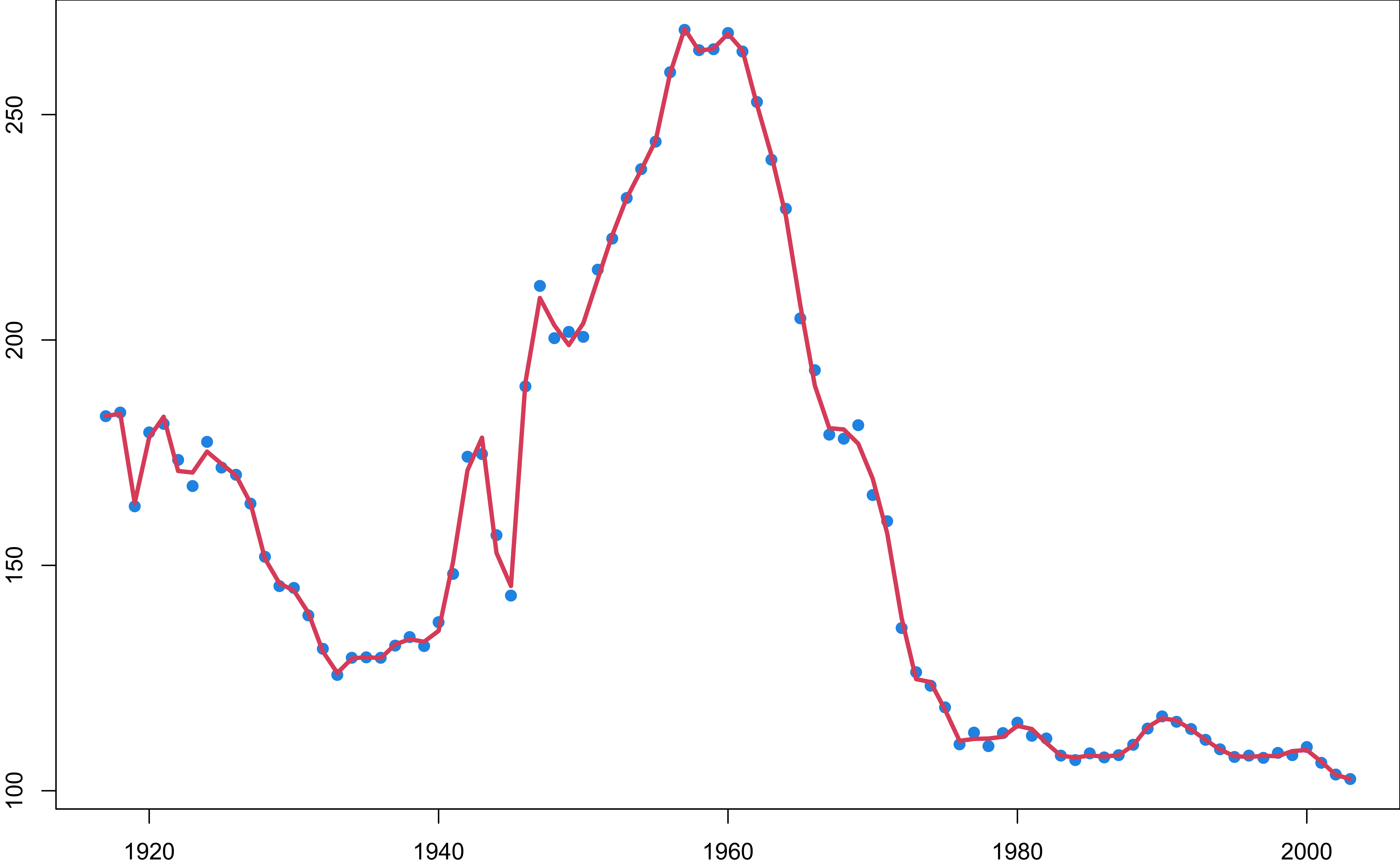
smooth.spline()
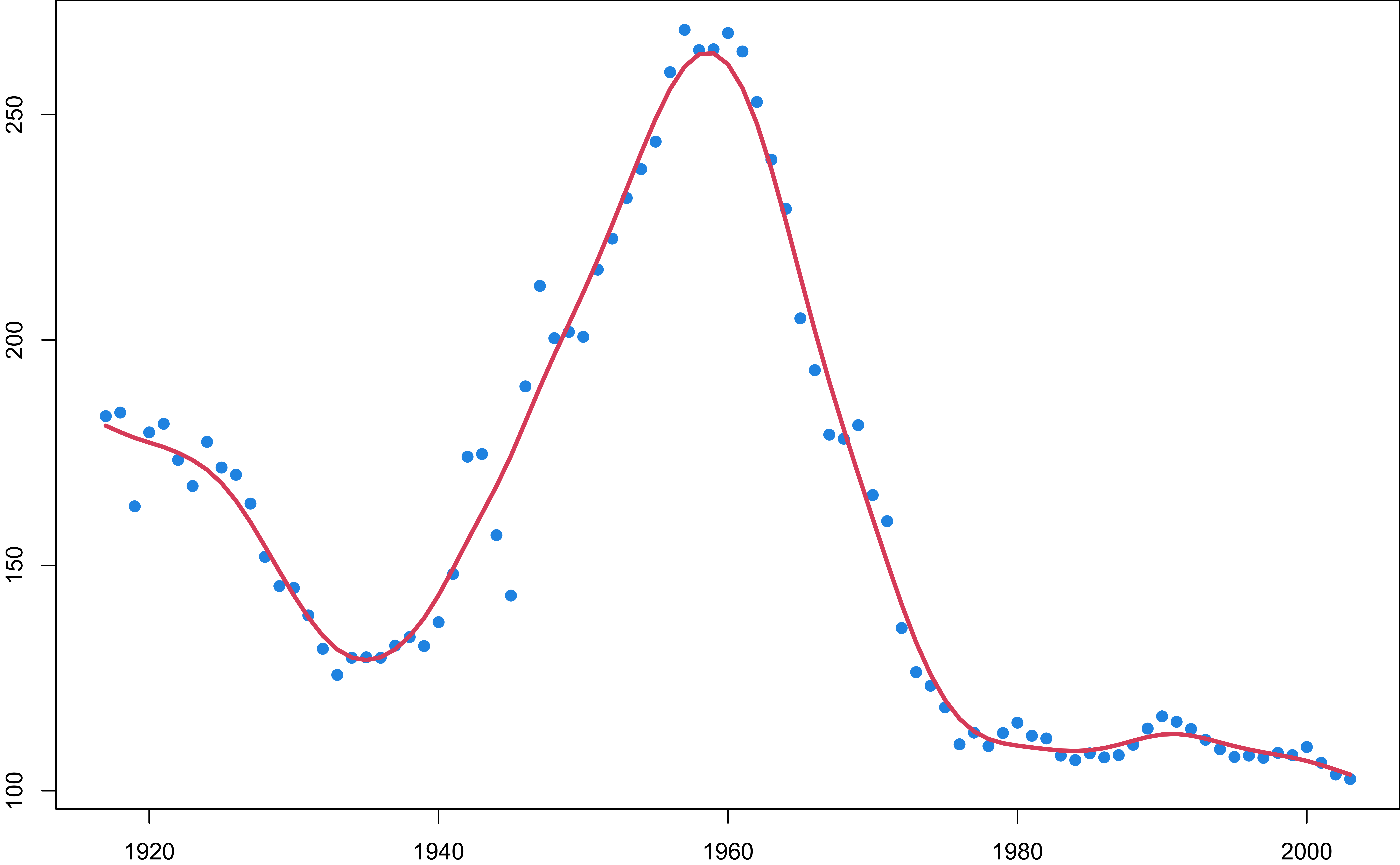
Generalized Additive Models
Extending Splines to Multiple Variables
All methods discussed so far are extensions of simple linear regression.
How to flexibly predict \(y\) or nonlinear regression function on the basis of several predictors \(x_1, \dots, x_p\)?
Maintaining the additive structure of linear models, but allowing nonlinear functions of each of the variables.
\[y = \beta_0 + f_1(x_1) + f_2(x_2) + \dots + f_p(x_p) + \epsilon\]
- This is a generalized additive model.
- It’s general: it can be modelling response with other distributions, binary, counts, positive values, for example.
- It’s additive: calculate a separate \(f_j\) for each \(x_j\), and add together all of their contributions.
- \(f_1(x_1) = x_1\); \(f_2(x_2) = x_2 + x_2^2\); \(f_3(x_3) = \text{cubic splines}\)
Wage data in ISL
Rows: 3,000
Columns: 11
$ year       <int> 2006, 2004, 2003, 2003, 2005, 2008, 2009, 2008, 2006, 2004,…
$ age        <int> 18, 24, 45, 43, 50, 54, 44, 30, 41, 52, 45, 34, 35, 39, 54,…
$ maritl     <fct> 1. Never Married, 1. Never Married, 2. Married, 2. Married,…
$ race       <fct> 1. White, 1. White, 1. White, 3. Asian, 1. White, 1. White,…
$ education  <fct> 1. < HS Grad, 4. College Grad, 3. Some College, 4. College …
$ region     <fct> 2. Middle Atlantic, 2. Middle Atlantic, 2. Middle Atlantic,…
$ jobclass   <fct> 1. Industrial, 2. Information, 1. Industrial, 2. Informatio…
$ health     <fct> 1. <=Good, 2. >=Very Good, 1. <=Good, 2. >=Very Good, 1. <=…
$ health_ins <fct> 2. No, 2. No, 1. Yes, 1. Yes, 1. Yes, 1. Yes, 1. Yes, 1. Ye…
$ logwage    <dbl> 4.32, 4.26, 4.88, 5.04, 4.32, 4.85, 5.13, 4.72, 4.78, 4.86,…
$ wage       <dbl> 75.0, 70.5, 131.0, 154.7, 75.0, 127.1, 169.5, 111.7, 118.9,…
gam::gam()
s()for smoothing splinesCoefficients not that interesting; fitted functions are.
