Generative Models

MSSC 6250 Statistical Machine Learning

Dr. Cheng-Han Yu
Department of Mathematical and Statistical Sciences
Marquette University

Background: Bayes Classifier

Bayes Classifier

The test error rate is minimized, on average, by a classifier that assigns each observation to the most likely category, given its predictor values.

This fact leads to

• Bayes (Optimal) Classifier: Assign a test observation \(y_j\) with predictor \(x_j\) to class \(k\) for which the conditional probability \(P(Y_j = k \mid X = x_j)\) is largest.

• The Bayes classifier produces the lowest possible test error rate, called Bayes error rate.

The problem is

• We never know \(P(Y_j = k \mid X = x_j)\) 😭

• The goal of soft classifiers is to estimate it, like logistic regression:

\[ \widehat{\pi}(\mathbf{x}) = \widehat{P}(Y = 1 \mid \mathbf{x}) = \frac{1}{1+e^{-\mathbf{x}'\widehat{\boldsymbol{\beta}}}}\]

[What is ``Bayes regression function”? In statistics, it is called oracle when a method/model has access to the ground truth.]

Generative Models

What is a Generative Model?

• So far predictors are assumed fixed and known, and we care about the conditional distribution, \(p(y \mid \mathbf{x})\)
  • Logistic regression (LR)

• A generative model considers the joint distribution of the response and predictors, i.e., \(p(y, \mathbf{x})\)
  • Discriminant analysis
  • Naive Bayes (NB)

Why not just logistic regression?

• When the classes are substaintially separated, the parameter estimates for the logistic regression are unstable.

• If the distribution of the predictors is approximately normal in each of the classes and the sample size is small, the generative models could perform better and more stable.

\(\mathbf{x}\) is variable whose value is generated from some distribution given a value of \(y\)

Generative Modeling

• To infer/predict \(p(y = k \mid \mathbf{x})\) from a generative model, Bayes theorem comes into play:

\[\begin{align} p(y = k \mid \mathbf{x}) &= \frac{p(y = k, \mathbf{x})}{p(\mathbf{x})} = \frac{p(y = k)p(\mathbf{x}\mid y = k) }{p(\mathbf{x})} = \frac{p(y = k)p(\mathbf{x}\mid y = k)}{\sum_{l=1}^K p(y = k)p(\mathbf{x}\mid y = l)}\\ &=\frac{\pi_kf_k(\mathbf{x})}{\sum_{l=1}^K\pi_lf_l(\mathbf{x})}\end{align}\]

• To get the posterior \(p(y = k \mid \mathbf{x})\), we need
  • prior \(\pi_k = p(y = k)\)
  • likelihood \(f_k(\mathbf{x}) = p(\mathbf{x}\mid y = k)\)

Note

Different generative models use different priors and likelihoods, resulting in different strengths and weakness.

Bayes Decision Boundary

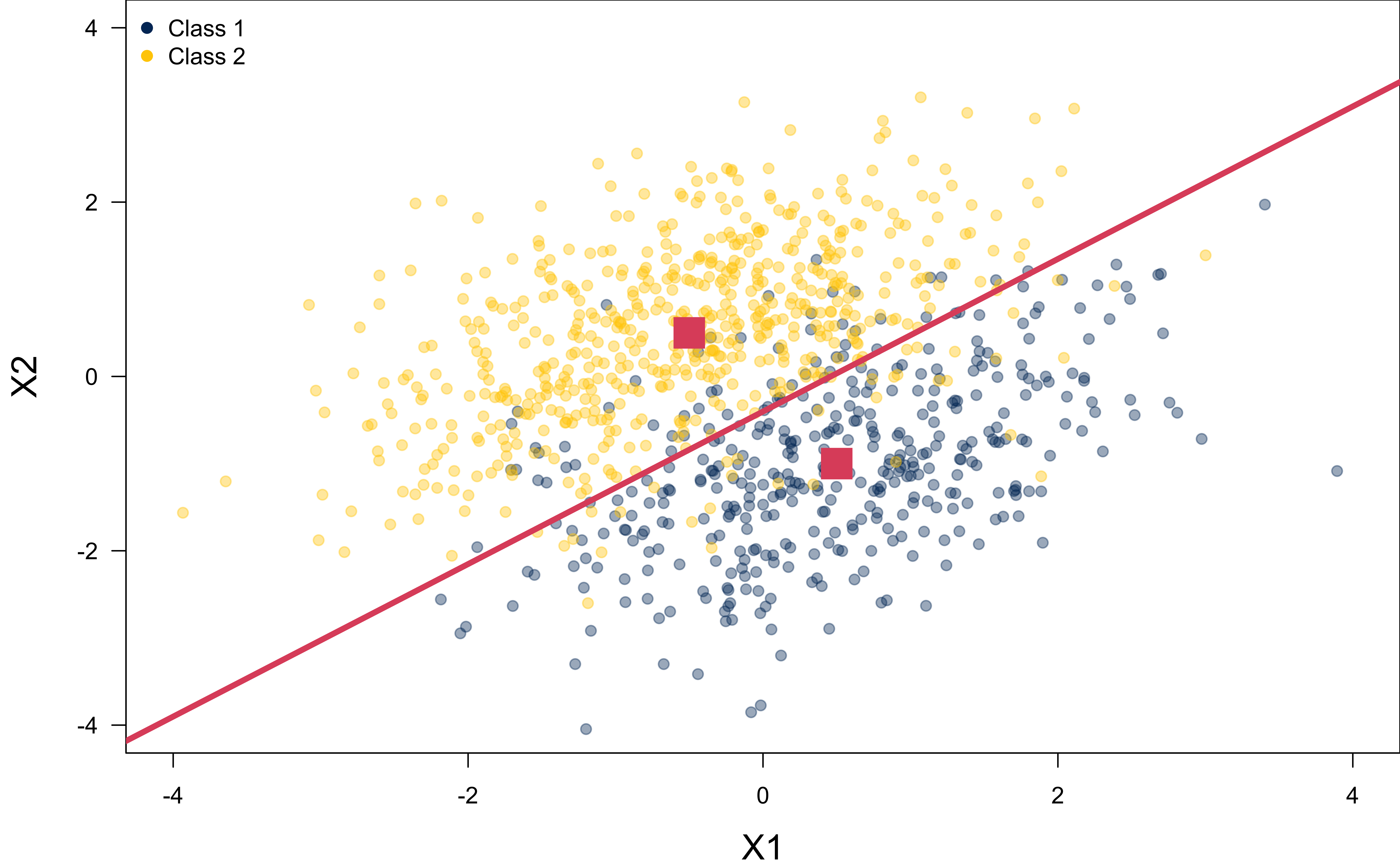
How do we find/estimate the Bayes decision boundary generated by the Bayes classifier?

Linear Discriminant Analysis (LDA)

\[\begin{align} p(y = k \mid \mathbf{x}) = \frac{p(y = k)p(\mathbf{x}\mid y = k)}{\sum_{l=1}^K p(y = k)p(\mathbf{x}\mid y = l)} =\frac{\pi_kf_k(\mathbf{x})}{\sum_{l=1}^K\pi_lf_l(\mathbf{x})}\end{align}\]

• Estimate the prior \(\pi_k = p(y = k)\) using the proportion of the training labels that belong to the \(k\)th class: \[\hat{\pi}_k = n_k / n \]

table(Default$default)/length(Default$default)

    No    Yes 
0.9667 0.0333 

• LDA assumption for \(f_k(\mathbf{x})\): \(\color{blue}{(\mathbf{x}\mid y = k) \sim N_p\left(\boldsymbol{\mu}_k, \Sigma \right)}\)
  • \(\boldsymbol{\mu}_k\): class-specific mean vector
  • \(\Sigma\): covariance matrix common to all \(K\) classes

Two Multivariate Normals with Common Covariance

\(\color{blue}{(\mathbf{x}\mid y = k) \sim N_p\left(\boldsymbol{\mu}_k, \Sigma \right)}\)

• \(\boldsymbol{\mu}_1 = (0.5, -1)'\), \(\boldsymbol{\mu}_2 = (-0.5, 0.5)'\)

• \(\Sigma = \begin{pmatrix} 1 & 0.5 \\ 0.5 & 1 \end{pmatrix}\)

• \(\pi_1 = 0.4\), \(\pi_2 = 0.6\)

• Each class has its own predictor mean.

• The predictor’s variability are the same for the two classes.

plot_ly has mu1 mu2 problems! Be careful!

Parameter Estimation for LDA

\(\color{blue}{(\mathbf{x}\mid y = k) \sim N_p\left(\boldsymbol{\mu}_k, \Sigma \right)}\)

• Estimating \(p(\mathbf{x}\mid y = k)\) is reduced to estimating \(\boldsymbol{\mu}_1, \dots, \boldsymbol{\mu}_K\) and \(\Sigma\).

• Centroid/sample mean: \(\widehat{\boldsymbol{\mu}}_k = \frac{1}{n_k} \sum_{i: \,y_i = k} \mathbf{x}_i\)
• Pooled covariance matrix: \[\widehat \Sigma = \frac{1}{n-K} \sum_{k=1}^K \sum_{i : \, y_i = k} (\mathbf{x}_i - \widehat{\boldsymbol{\mu}}_k) (\mathbf{x}_i - \widehat{\boldsymbol{\mu}}_k)' = \sum_{k=1}^K \frac{n_k-1}{n-K}\widehat \Sigma_k\] where \(\widehat \Sigma_k = \frac{1}{n_k-1}\sum_{i : \, y_i = k} (\mathbf{x}_i - \widehat{\boldsymbol{\mu}}_k) (\mathbf{x}_i - \widehat{\boldsymbol{\mu}}_k)'\)

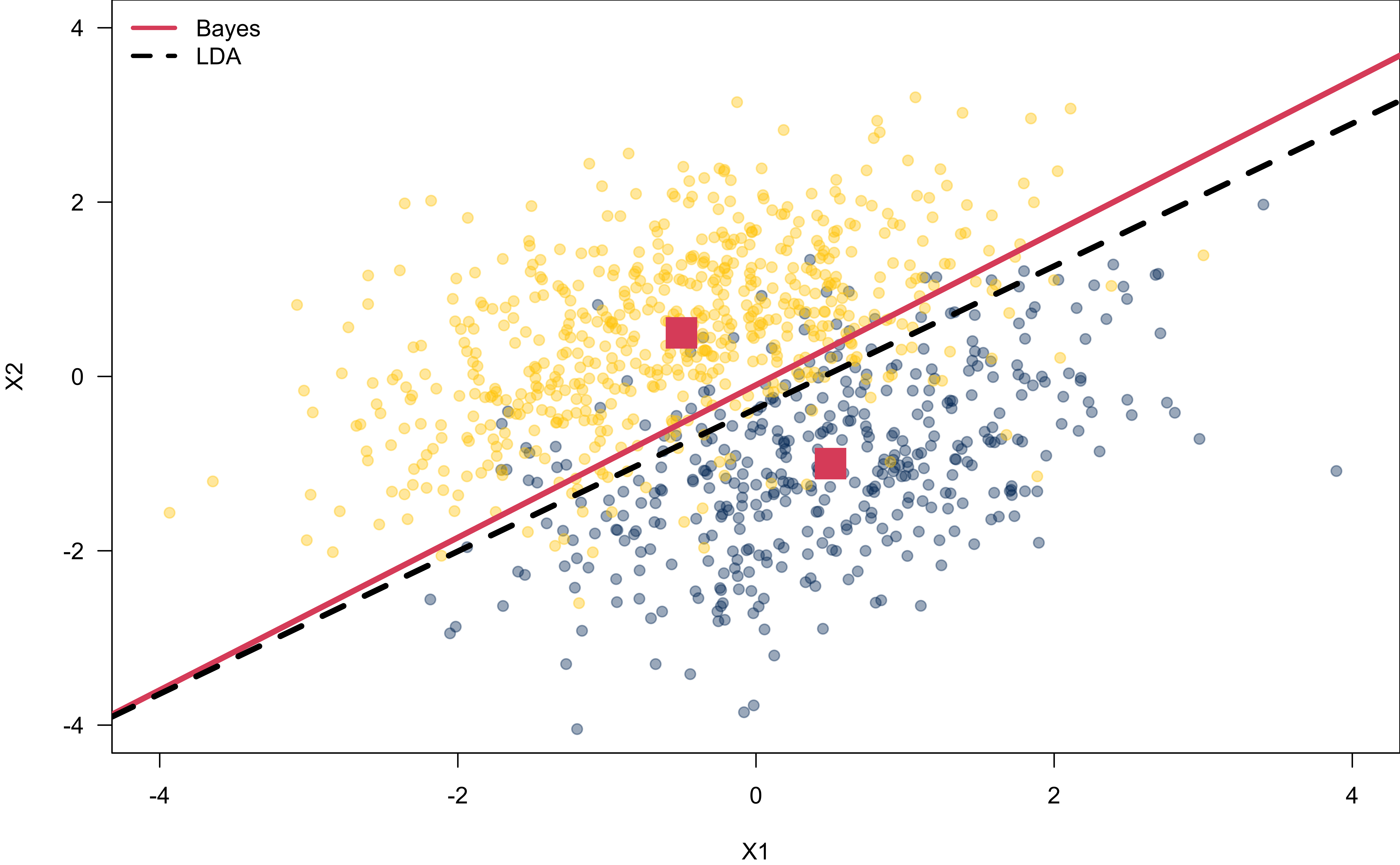
mu1_hat =

[1]  0.47 -1.01

mu2_hat =

[1] -0.54  0.51

Sigma_hat = 

     [,1] [,2]
[1,] 1.13 0.54
[2,] 0.54 1.02

Decision Boundary by LDA

Discriminant Function

The likelihood is Gaussian

\[f_k(x) = \frac{1}{(2\pi)^{p/2} |\Sigma|^{1/2}} \exp\left[ -\frac{1}{2} (\mathbf{x}- \boldsymbol{\mu}_k)' \Sigma^{-1} (\mathbf{x}- \boldsymbol{\mu}_k) \right]\]

The log-likelihood is

\[\begin{align} \log f_k(\mathbf{x}) =&~ -\log \big((2\pi)^{p/2} |\Sigma|^{1/2} \big) - \frac{1}{2} (\mathbf{x}- \boldsymbol{\mu}_k)'\Sigma^{-1} (\mathbf{x}- \boldsymbol{\mu}_k) \\ =&~ - \frac{1}{2} (\mathbf{x}- \boldsymbol{\mu}_k)' \Sigma^{-1} (\mathbf{x}- \boldsymbol{\mu}_k) + \text{Constant} \end{align}\]

The maximum a posteriori estimate is

\[\begin{align} \widehat f(\mathbf{x}) =& ~\underset{k}{\arg\max} \,\, \log \big( \pi_k f_k(\mathbf{x}) \big) \\ =& ~\underset{k}{\arg\max} \,\, - \frac{1}{2} (\mathbf{x}- \boldsymbol{\mu}_k)' \Sigma^{-1} (\mathbf{x}- \boldsymbol{\mu}_k) + \log(\pi_k) \end{align}\]

Discriminant Function

\[\begin{align} \widehat f(\mathbf{x}) =& ~\underset{k}{\arg\max} \,\, - \frac{1}{2} (\mathbf{x}- \boldsymbol{\mu}_k)' \Sigma^{-1} (\mathbf{x}- \boldsymbol{\mu}_k) + \log(\pi_k) \end{align}\]

• \((\mathbf{x}- \boldsymbol{\mu}_k)' \Sigma^{-1} (\mathbf{x}- \boldsymbol{\mu}_k)\) is the Mahalanobis distance between \(\mathbf{x}\) and the centroid \(\boldsymbol{\mu}_k\).
• Classify \(y\) so that its \(\mathbf{x}\) and the centroid of the labeled class is the closest (after adjusting the for prior). \[\begin{align} & - \frac{1}{2} (\mathbf{x}- \boldsymbol{\mu}_k)' \Sigma^{-1} (\mathbf{x}- \boldsymbol{\mu}_k) + \log(\pi_k)\\ &=~ \mathbf{x}' \underbrace{\Sigma^{-1} \boldsymbol{\mu}_k}_{\mathbf{w}_k} \underbrace{- \frac{1}{2}\boldsymbol{\mu}_k' \Sigma^{-1} \boldsymbol{\mu}_k + \log(\pi_k)}_{b_k} + \text{const of } k \\ &=~ \mathbf{x}' \mathbf{w}_k + b_k + \text{const of } k\\ &=~ \delta_k(\mathbf{x}) + \text{const of } k \end{align}\] where \(\delta_k(\mathbf{x})\) the discriminant function which is linear in \(\mathbf{x}\).

by incorporating the covariance matrix and adjusting the for prior. Note that anything that does not depends on the class index \(k\) is irrelevant to the decision.

Discriminant Function

• The decision boundary of LDA is a linear function of \(\mathbf{x}\).

• The boundary between two classes \(k\) and \(l\) is where they have the same density value.

\[\begin{align} \delta_k(\mathbf{x}) &= \delta_l(\mathbf{x}) \\ \Leftrightarrow \quad \mathbf{x}' \mathbf{w}_k + b_k &= \mathbf{x}' \mathbf{w}_l + b_l \\ \Leftrightarrow \quad \mathbf{x}' (\mathbf{w}_k - \mathbf{w}_l) + (b_k - b_l) &= 0. \\ \end{align}\]

\[\begin{align} &\delta_k(\mathbf{x}) - \delta_l(\mathbf{x}) \\ \propto & \quad \log \left(\pi_k f_k(\mathbf{x})\right) - \log \left(\pi_l f_l(\mathbf{x}))\right)\\ \propto & \quad \log \left(P(Y = k \mid \mathbf{x})\right) - \log \left(P(Y = l \mid \mathbf{x})\right) \\ \propto & \quad \log \left( \frac{P(Y = k \mid \mathbf{x})}{P(Y = l \mid \mathbf{x})}\right) \end{align}\]

Interpretation of LDA

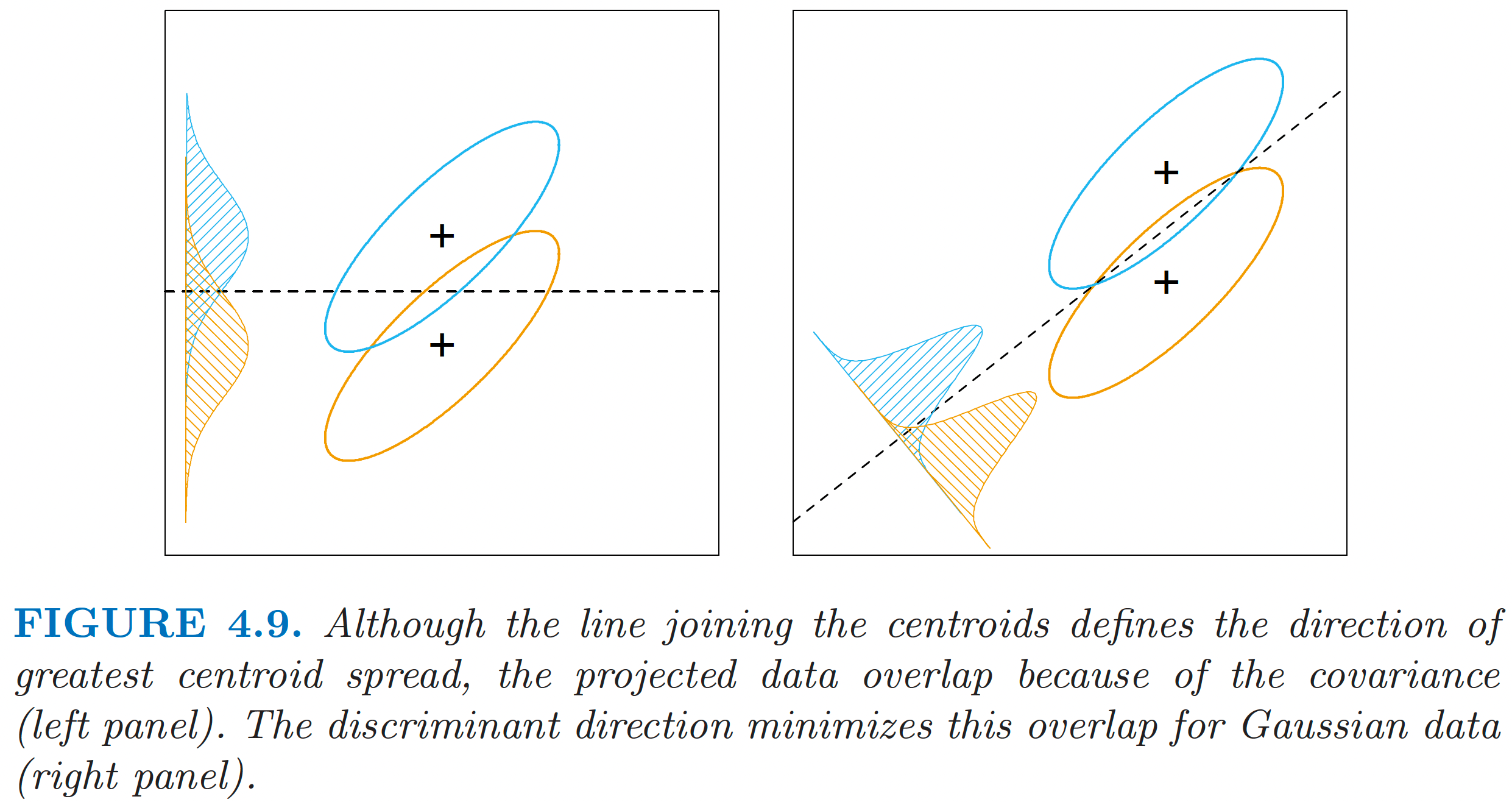
ESL Fig 4.9

Check ESL

Find the linear combination \(Z = a'X\) such that the between class variance is maximized relative to the within-class variance.

Again, the between class variance is the variance of the class means of Z, and the within class variance is the pooled variance about the means. Figure 4.9 shows why this criterion makes sense. Although the direction joining the centroids separates the means as much as possible (i.e., maximizes the between-class variance), there is considerable overlap between the projected classes due to the nature of the covariances. By taking the covariance into account as well, a direction with minimum overlap can be found.

Gaussian classification with common covariances leads to linear decision boundaries. Classification can be achieved by sphering the data with respect to W, and classifying to the closest centroid (modulo log πk) in the sphered space. Since only the relative distances to the centroids count, one can confine the data to the subspace spanned by the centroids in the sphered space. This subspace can be further decomposed into successively optimal subspaces in term of centroid separation. This decomposition is identical to the decomposition due to Fisher.

MASS::lda()

LDA

lda_fit <- MASS::lda(default ~ balance, data = Default)
lda_pred <- predict(lda_fit, data = Default)
(lda_conf <- table(lda_pred$class, Default$default))

     
        No  Yes
  No  9643  257
  Yes   24   76

• training accuracy is 0.972
• sensitivity is 0.228

Logistic Regression

       
          No  Yes
  FALSE 9625  233
  TRUE    42  100

• training accuracy is 0.973
• sensitivity is 0.3

Quadratic Discriminant Analysis (QDA)

• LDA assumption for \(f_k(\mathbf{x})\): \(\color{blue}{(\mathbf{x}\mid y = k) \sim N_p\left(\boldsymbol{\mu}_k, \Sigma \right)}\)
  • \(\Sigma\): covariance matrix common to all K classes

• QDA assumption for \(f_k(\mathbf{x})\): \(\color{blue}{(\mathbf{x}\mid y = k) \sim N_p\left(\boldsymbol{\mu}_k, \Sigma_k \right)}\)
  • \(\Sigma_k\): each class has its own covariance matrix

The discriminant function for QDA is

\[\begin{align} \delta_k(\mathbf{x}) &= - \frac{1}{2} (\mathbf{x}- \boldsymbol{\mu}_k)' \Sigma_k^{-1} (\mathbf{x}- \boldsymbol{\mu}_k) - \frac{1}{2} \log |\Sigma_k |+ \log(\pi_k) \\ &= \mathbf{x}' \mathbf{W}_k \mathbf{x}+ \mathbf{x}'\mathbf{w}_k + b_k \end{align}\] which is a quadratic function of \(\mathbf{x}\).

The boundary between class \(k\) and \(l\) for QDA is

\[\begin{align} \mathbf{x}' (\mathbf{W}_k - \mathbf{W}_l) \mathbf{x}+ \mathbf{x}' (\mathbf{w}_k - \mathbf{w}_l) + (b_k - b_l) = 0\\ \end{align}\]

Parameter Estimation for QDA

The estimation procedure is almost the same as LDA.

• \(\hat{\pi}_k = n_k / n\)

• Centroids: \(\widehat{\boldsymbol{\mu}}_k = \frac{1}{n_k} \sum_{i: \,y_i = k} \mathbf{x}_i\)

• Individual covariance matrix: \[\widehat \Sigma_k = \frac{1}{n_k-1}\sum_{i : \, y_i = k} (\mathbf{x}_i - \widehat{\boldsymbol{\mu}}_k) (\mathbf{x}_i - \widehat{\boldsymbol{\mu}}_k)'\]

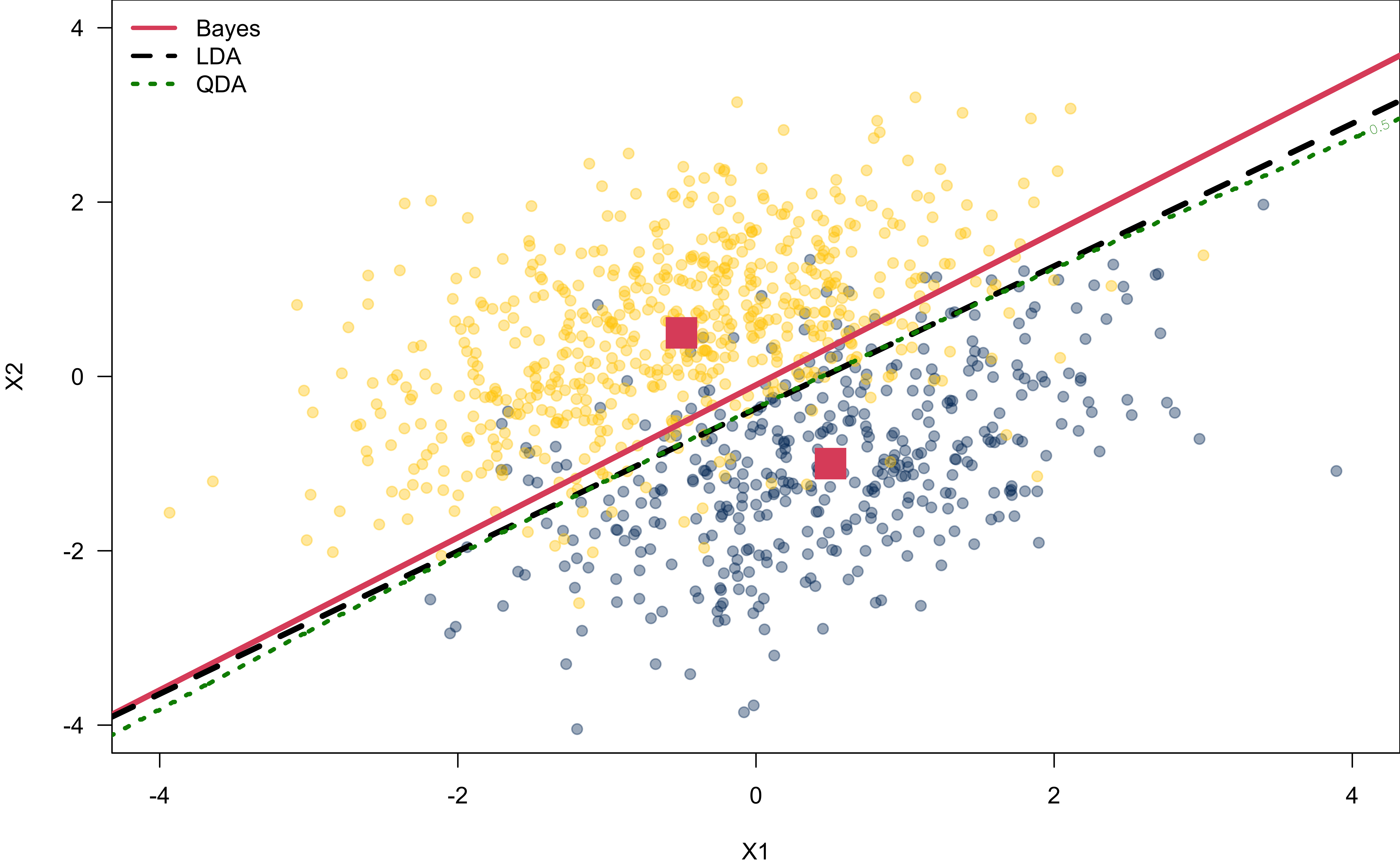
Two Multivariate Normals with Different Covariance Matrices

\(\color{blue}{(\mathbf{x}\mid y = k) \sim N_p\left(\boldsymbol{\mu}_k, \Sigma_k \right)}\)

• \(\boldsymbol{\mu}_1 = (0.5, -1)'\)

• \(\boldsymbol{\mu}_2 = (-0.5, 0.5)'\)

• \(\Sigma_1 = \begin{pmatrix} 1 & 0.5 \\ 0.5 & 1 \end{pmatrix}\)

• \(\Sigma_2 = \begin{pmatrix} 1 & -0.5 \\ -0.5 & 1 \end{pmatrix}\)

• \(\pi_1 = 0.4\), \(\pi_2 = 0.6\)

• Each class has its own predictor mean and covariance matrix.

Decision Boundary by QDA

https://freakonometrics.hypotheses.org/tag/qda

MASS::qda

LDA

     
        No  Yes
  No  9643  257
  Yes   24   76

QDA

qda_fit <- MASS::qda(default ~ balance, data = Default)
qda_pred <- predict(qda_fit, data = Default)
(qda_conf <- table(qda_pred$class, Default$default))

     
        No  Yes
  No  9639  246
  Yes   28   87

• training accuracy is 0.973
• sensitivity is 0.261

Naive Bayes (NB)

• LDA assumption for \(f_k(\mathbf{x})\): \(\color{blue}{(\mathbf{x}\mid y = k) \sim N_p\left(\boldsymbol{\mu}_k, \Sigma \right)}\)
  • \(\Sigma\): covariance matrix common to all K classes

• QDA assumption for \(f_k(\mathbf{x})\): \(\color{blue}{(\mathbf{x}\mid y = k) \sim N_p\left(\boldsymbol{\mu}_k, \Sigma_k \right)}\)
  • \(\Sigma_k\): each class has its own covariance matrix

• NB assumption for \(f_k(\mathbf{x})\):
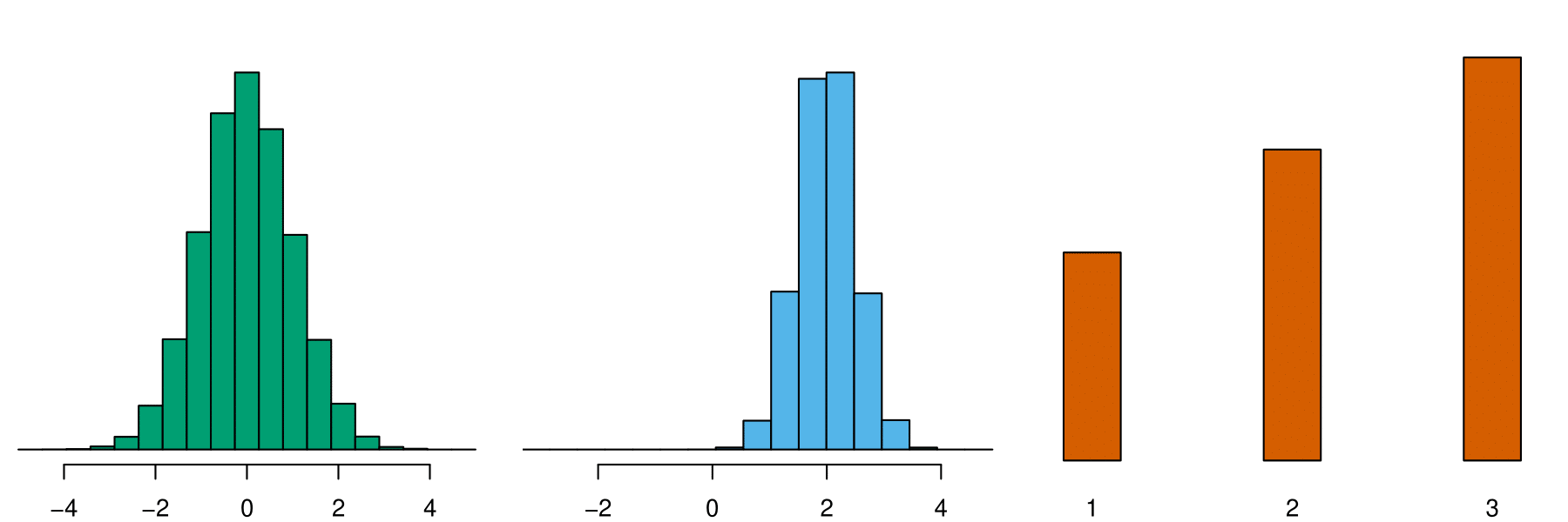
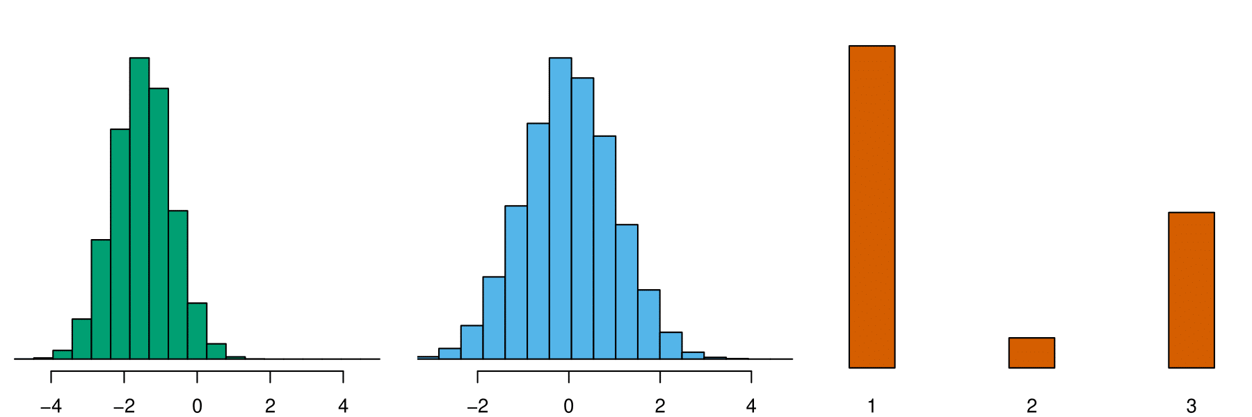
  • features within each class are independent!
  • \(f_k(\mathbf{x}) = f_{k1}(x_1) \times f_{k2}(x_2) \times \cdots \times f_{kp}(x_p)\)

• Considering the joint distribution of predictors is a pain when \(p\) is large.

• We don’t believe \(p\) predictors are not associated at all, but this “naive” assumption leads to decent results when \(n\) is not large enough relative to \(p\).

• The naive independence assumption introduces some bias, but reduces variance.

\[\begin{align} p(y = k \mid \mathbf{x}) =\frac{\pi_kf_k(\mathbf{x})}{\sum_{l=1}^K\pi_lf_l(\mathbf{x})} = \frac{\pi_k\prod_{j=1}^p f_{kj(x_j)}}{\sum_{l=1}^K\pi_l\prod_{j=1}^p f_{lj(x_j)}} \end{align}\]

estimating a joint distribution requires such a huge amount of data

Options for Estimating \(f_{kj}(x_j)\)

• Numerical \(X_j\)
  • Parametric: \[(X_j \mid Y = k) \sim N\left(\mu_{jk}, \sigma_{jk}^2 \right).\] It’s QDA with additional assumption that \(\Sigma_k\) is diagonal.
  • Non-parametric: Estimate \(f_{kj}(x_j)\) by (discrete) histogram, (continuous) kernel density estimator, etc.

• Categorical \(X_j\)

  • \(f_{kj}(x_j) \approx\) the proportion of training data for \(x_j\) corresponding to class \(k\).

Class 1

Class 2

ISL Fig. 4.10. Left to right: estimated density of \(x_1\), \(x_2\) and estimated probability of \(x_3\).

e1071::naiveBayes()

QDA

     
        No  Yes
  No  9639  246
  Yes   28   87

Naive Bayes - By default, each feature is Gaussian distributed.

nb_fit <- e1071::naiveBayes(default ~ balance, data = Default)
nb_pred <- predict(nb_fit, Default)
(nb_conf <- table(nb_pred, Default$default))

       
nb_pred   No  Yes
    No  9639  246
    Yes   28   87

• training accuracy is 0.973
• sensitivity is 0.261

Comparison of Classification Methods (LR, LDA, QDA, NB)

Log Odds of LR and LDA

Suppose class \(K\) is the baseline.

• LR

\[\log \left( \frac{P(Y = k \mid \mathbf{x})}{P(Y = K \mid \mathbf{x})}\right) = \beta_{k0} + \beta_{k1}x_{1} + \dots + \beta_{kp}x_{p}\]

• LDA

\[\log \left( \frac{P(Y = k \mid \mathbf{x})}{P(Y = K \mid \mathbf{x})}\right) = a_k + \sum_{j=1}^pc_{kj}x_j\] where \(a_k = \log(\pi_k / \pi_K) - \frac{1}{2}(\boldsymbol{\mu}_k + \boldsymbol{\mu}_K)'\Sigma^{-1}(\boldsymbol{\mu}_k - \boldsymbol{\mu}_K)\) and \(c_{kj}\) is the \(j\)th element of \(\Sigma^{-1}(\boldsymbol{\mu}_k - \boldsymbol{\mu}_K)\).

Both log odds are linear in \(\mathbf{x}\).

Log Odds of QDA and NB

• QDA

\[\log \left( \frac{P(Y = k \mid \mathbf{x})}{P(Y = K \mid \mathbf{x})}\right) = a_k + \sum_{j=1}^pc_{kj}x_j + \sum_{j=1}^p\sum_{l=1}^p d_{kjl}x_jx_l\] The log odds is quadratic in \(\mathbf{x}\), where \(a_k\), \(c_{kj}\) and \(d_{kjl}\) are functions of \(\pi_k\), \(\pi_K\), \(\boldsymbol{\mu}_k\), \(\boldsymbol{\mu}_K\), \(\Sigma_k\) and \(\Sigma_K\).

• NB

\[\log \left( \frac{P(Y = k \mid \mathbf{x})}{P(Y = K \mid \mathbf{x})}\right) = a_k + \sum_{j=1}^pg_{kj}(x_j)\] where \(a_k = \log(\pi_k / \pi_K)\) and \(g_{kj}(x_j) = \log\left( \frac{f_{kj}(x_j)}{f_{Kj}(x_j)}\right)\).

The log odds takes the form of a generalized additive model!

Comparison of Log Odds

• LDA is a special case of QDA with \(d_{kjl} = 0\) for all \(k, j\) and \(l\). \((\Sigma_1 = \cdots = \Sigma_k = \Sigma)\)

• Any classifier with a linear decision boundary is a special case of NB with \(g_{kj}(x_j) = c_{kj}x_j.\)

  • LDA is a special case of NB. Really !? 😲

• NB is a special case of LDA if \(f_{kj}(x_j) = N\left(\mu_{jk}, \sigma_{j}^2 \right)\). \((\Sigma = \text{diag}(\sigma_1^2, \dots, \sigma_p^2))\)

• Neither QDA nor NB is a special case of the other

  • NB is more
    • flexible for any transformation of \(x_j\), \(g_{kj}(x_j)\).
    • restrictive because of its pure additive fit with no quadratic interactions \(d_{kjl}x_jx_l\).

Which Method to Use

• None of these methods uniformly dominates the others.

• The choice of method depends on

  • the true distribution of \(X_j\)s in each class
  • the sizes of \(n\) and \(p\) that controls bias-variance trade-off

• LDA outperforms LR when predictors are approximately normal, but use LR when inputs are away from normal.

• Use LDA but not QDA when variability of predictors are similar among all \(K\) classes.

• Do not use naive Bayes when predictors are clearly correlated.

• Use QDA when predictors clearly have different covariance structure for each class.

• LDA outperforms LR when predictors are approximately normal, but use LR when data are away from normal.

• Use LDA but not QDA when variability of predictors are similar among all \(K\) classes. QDA fits a more flexible classifier than necessary.

• Do not use naive Bayes when predictors are clearly correlated.

• Use QDA when predictors clearly have different covariance structure for each class.

Which Method to Use

• QDA is more flexible than LDA (more parameters to be estimated), and hence low bias and high variance.

• LDA tends to be better than QDA if \(n\) is relatively small, and so reducing variance is crucial.

• QDA is recommended if \(n\) is relatively large so that the variance of the classifier is not a major concern.

• Naive Bayes works when \(n\) is not large enough relative to \(p\).

\(n\) small more bias; \(p\) small less bias small \(n\) large \(p\): low bias high variance, so reducing variance by using less flexible method