K-nearest Neighbors

MSSC 6250 Statistical Machine Learning

Dr. Cheng-Han Yu
Department of Mathematical and Statistical Sciences
Marquette University

Nonparametric Examplar-based Methods

• So far we have mostly focused on parametric models, either unconditional \(p({\bf y} \mid \boldsymbol \theta)\) or conditional \(p({\bf y} \mid \mathbf{x}, \boldsymbol \theta)\), where \(\boldsymbol \theta\) is a fixed-dimensional vector of parameters. ¹

• The parameters are estimated from the training set \(\mathcal{D} = \{(\mathbf{x}_i, \mathbf{y}_i)\}_{i=1}^n\) but after model fitting, the data is not used anymore.

• The nonparametric models that keep the training data around at the test time are called examplar-based models, instance-based learning or memory-based learning.
  • K-nearest neighbors classification and regression
  • Kernel regression
  • Local regression, e.g., LOESS
  • Kernel density estimation

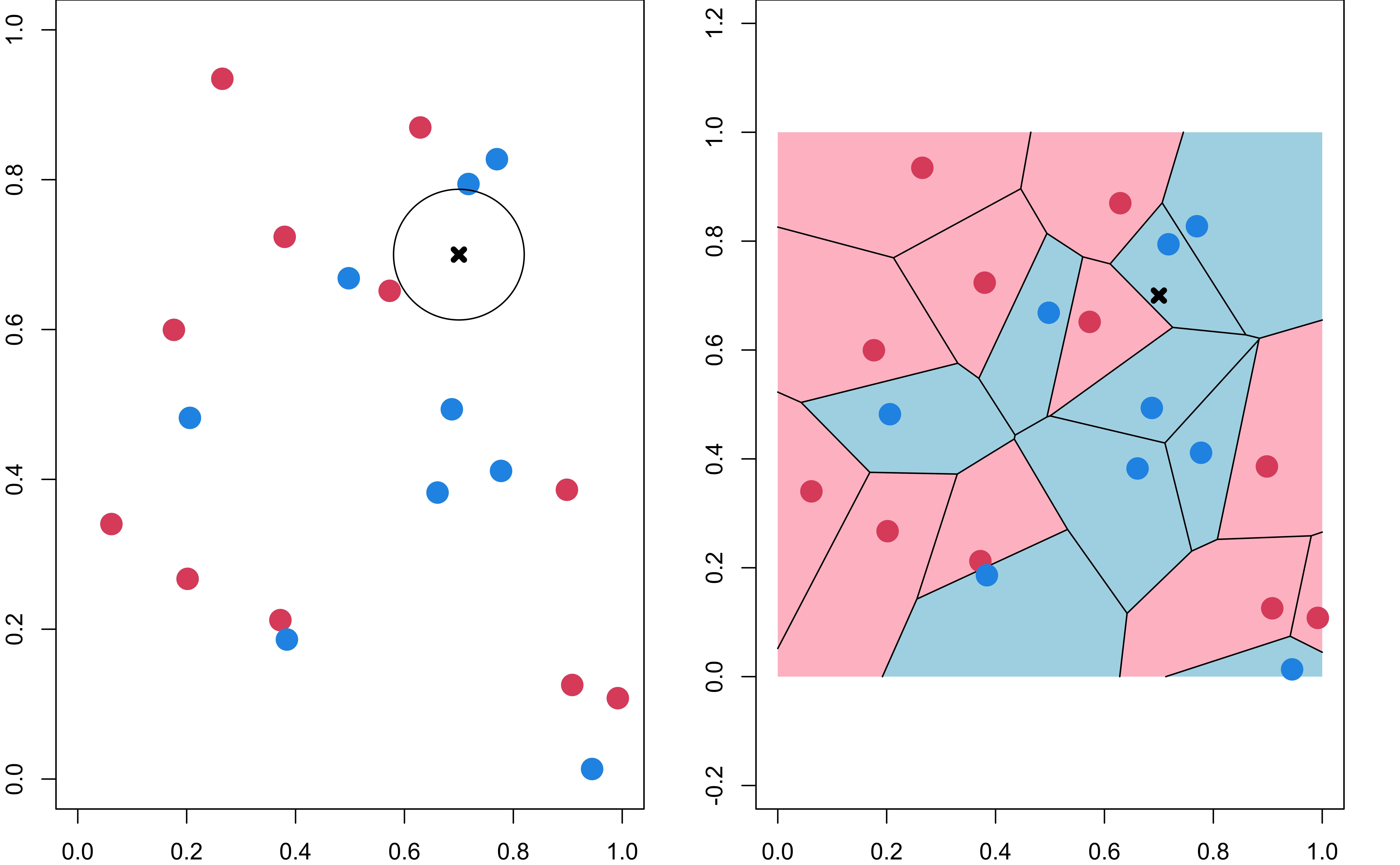
• The examplar-based models usually perform a local averaging technique based on the similarity or distance between a test input \(\mathbf{x}_0\) and each of the training inputs \(\mathbf{x}_i\).

1. For example, \(\beta\) coefficients in linear regression.

K-nearest Neighbor Regression

• K-nearest neighbor (KNN) is a nonparametric method.

• It can be used for both regression and classification.

• In KNN, we don’t have parameters \(\boldsymbol \beta\), and \(f(\mathbf{x}_0) = \mathbf{x}_0'\boldsymbol \beta\) in regression.¹

• We directly estimate \(f(\mathbf{x}_0)\) using our examples or memory.

\[ \widehat{y}_0 = \frac{1}{k} \sum_{x_i \in N_k(x_0)} y_i,\] where the neighborhood of \(x_0\), \(N_k(x_0)\), defines the \(k\) training data points that are closest to \(x_0\).

• Closeness (Similarity) is defined using a distance measure, such as the Euclidean distance.

1. \(\widehat{y}_0 = \widehat{f}(x_0)\).

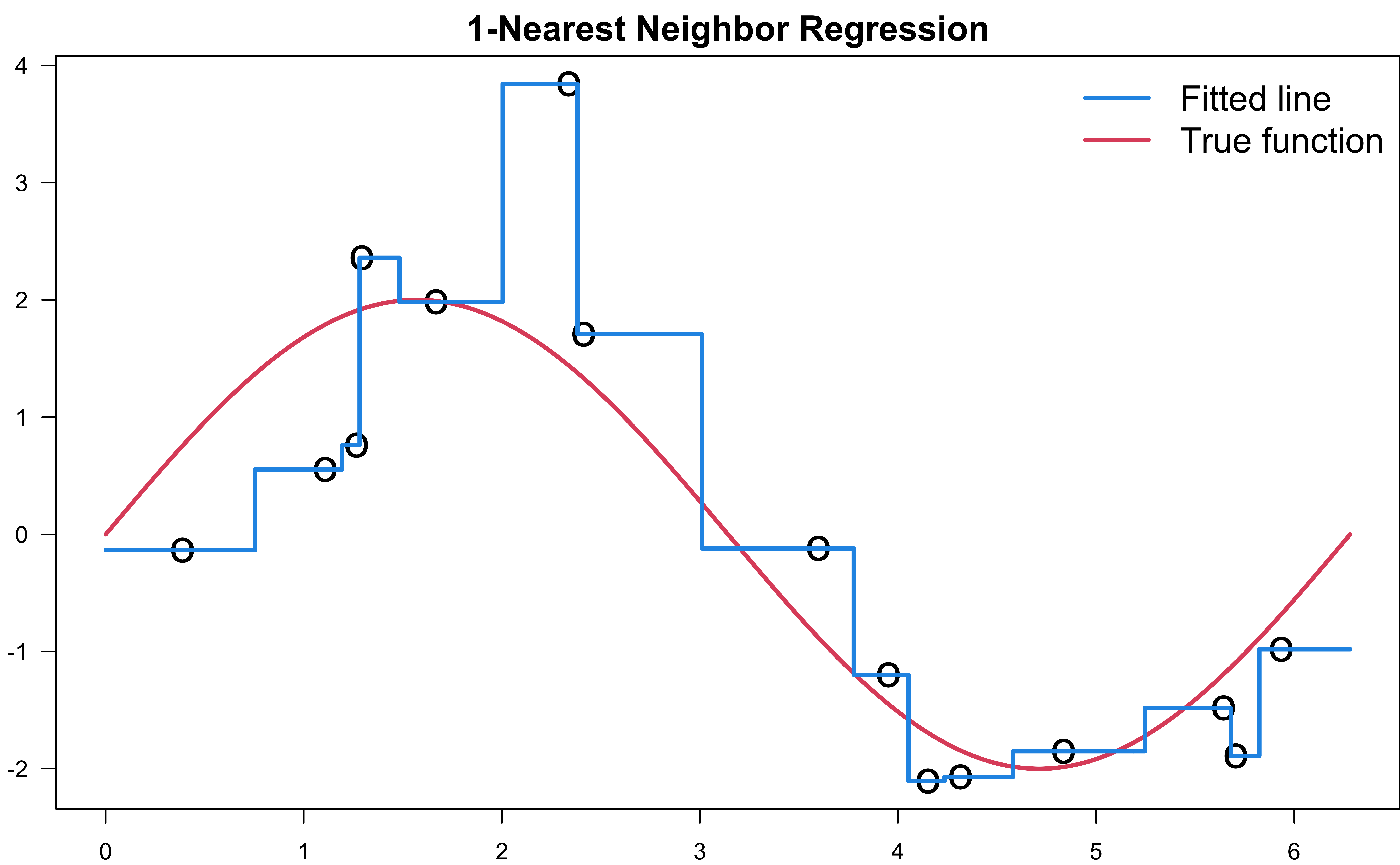
1-Nearest Neighbor Regression

Tuning \(k\)

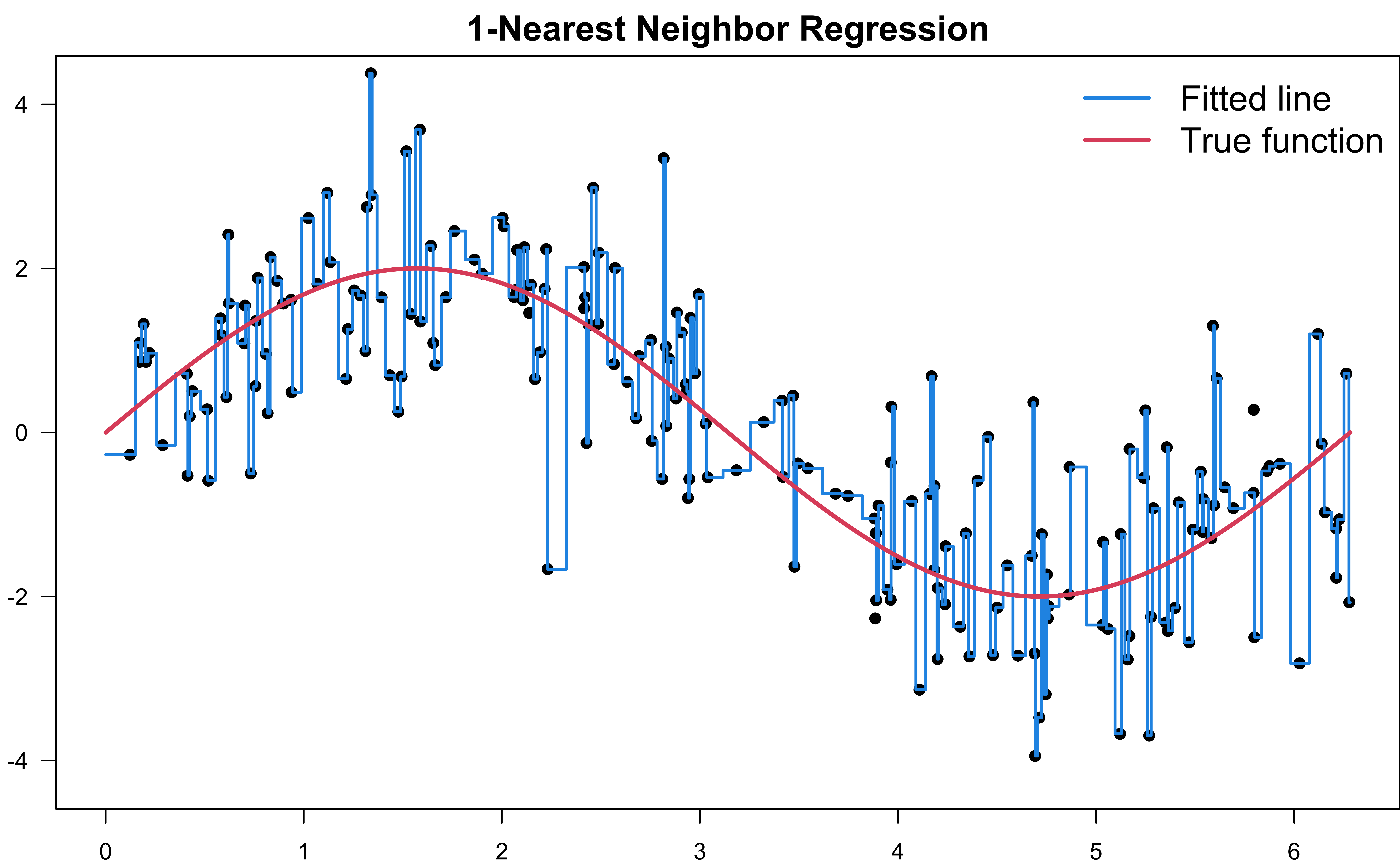
• \(y_i = 2\sin(x_i) + \epsilon_i, \quad \epsilon_i \stackrel{iid}{\sim} N(0, 1), \quad i = 1, \dots, 200\)

• put all weights on one single training point. The predictive value at some test \(x\) relies solely on one single training point that is closest to \(x\).

The Bias-variance Trade-off

If we consider different values of \(k\), we can observe the trade-off between bias and variance.

Bias-Variance Trade-Off

\[\begin{aligned} \text{E}\Big[ \big( Y - \widehat f(x_0) \big)^2 \Big] &= \underbrace{\text{E}\Big[ ( Y - f(x_0))^2 \big]}_{\text{Irreducible Error}} + \underbrace{\Big(f(x_0) - \text{E}[\widehat f(x_0)]\Big)^2}_{\text{Bias}^2} + \underbrace{\text{E}\Big[ \big(\widehat f(x_0) - \text{E}[\widehat f(x_0)] \big)^2 \Big]}_{\text{Variance}} \end{aligned}\]

• As \(k \uparrow\), bias \(\uparrow\) and variance \(\downarrow\) (smoother)
• As \(k \downarrow\), bias \(\downarrow\) and variance \(\uparrow\) (more wiggly)

when k is small, the estimated model is unstable. Also, each time we observe a new training data, we may get a very different estimation. (due to the closest sample and ) When k is large, the estimated model eventually deviates (systematically) from the truth. If we use more “neighbouring” points, say k, the variance would reduce to approximately σ2/k. But the bias2 will increase as neighbours are far away from x0. k determines the model complexity

Degrees of Freedom

• \(k\) determines the model complexity and degrees of freedom (df).

• In general, the df can be defined as

\[\text{df}(\hat{f}) = \frac{1}{\sigma^2}\text{Trace}\left( \mathrm{Cov}(\hat{\mathbf{y}}, \mathbf{y})\right)= \frac{1}{\sigma^2}\sum_{i=1}^n \mathrm{Cov}(\hat{y}_i, y_i)\]

• \(k = 1\): \(\hat{f}(x_i) = y_i\) and \(\text{df}(\hat{f}) = n\)

• \(k = n\): \(\hat{f}(x_i) = \bar{y}\) and \(\text{df}(\hat{f}) = 1\)

• For general \(k\), \(\text{df}(\hat{f}) = n/k\).

• Linear regression with \(p\) coefficients: \(\text{df}(\hat{f}) = \text{Trace}\left( {\bf H} \right) = p\)

• For any linear smoother \(\hat{\mathbf{y}} = {\bf S} \mathbf{y}\), \(\text{df}(\hat{f}) = \text{Trace}({\bf S})\).

K-nearest Neighbor Classification

• Instead of taking average in regression, KNN classification uses majority voting:

Look for the most popular class label among its neighbors.

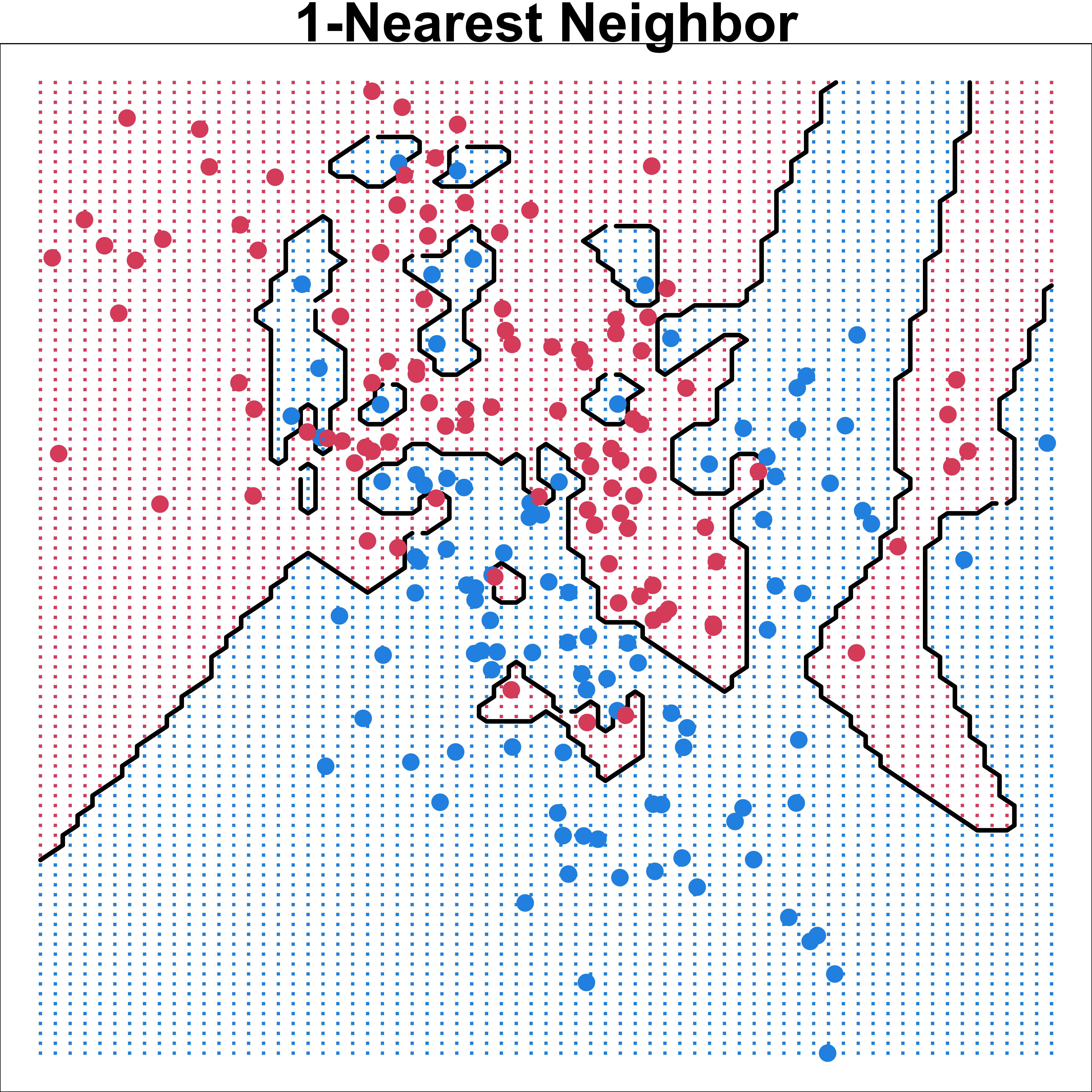
• 1NN decision boundary is a Voronoi diagram.

• Voronoi tessellation. https://en.wikipedia.org/wiki/Voronoi_diagram

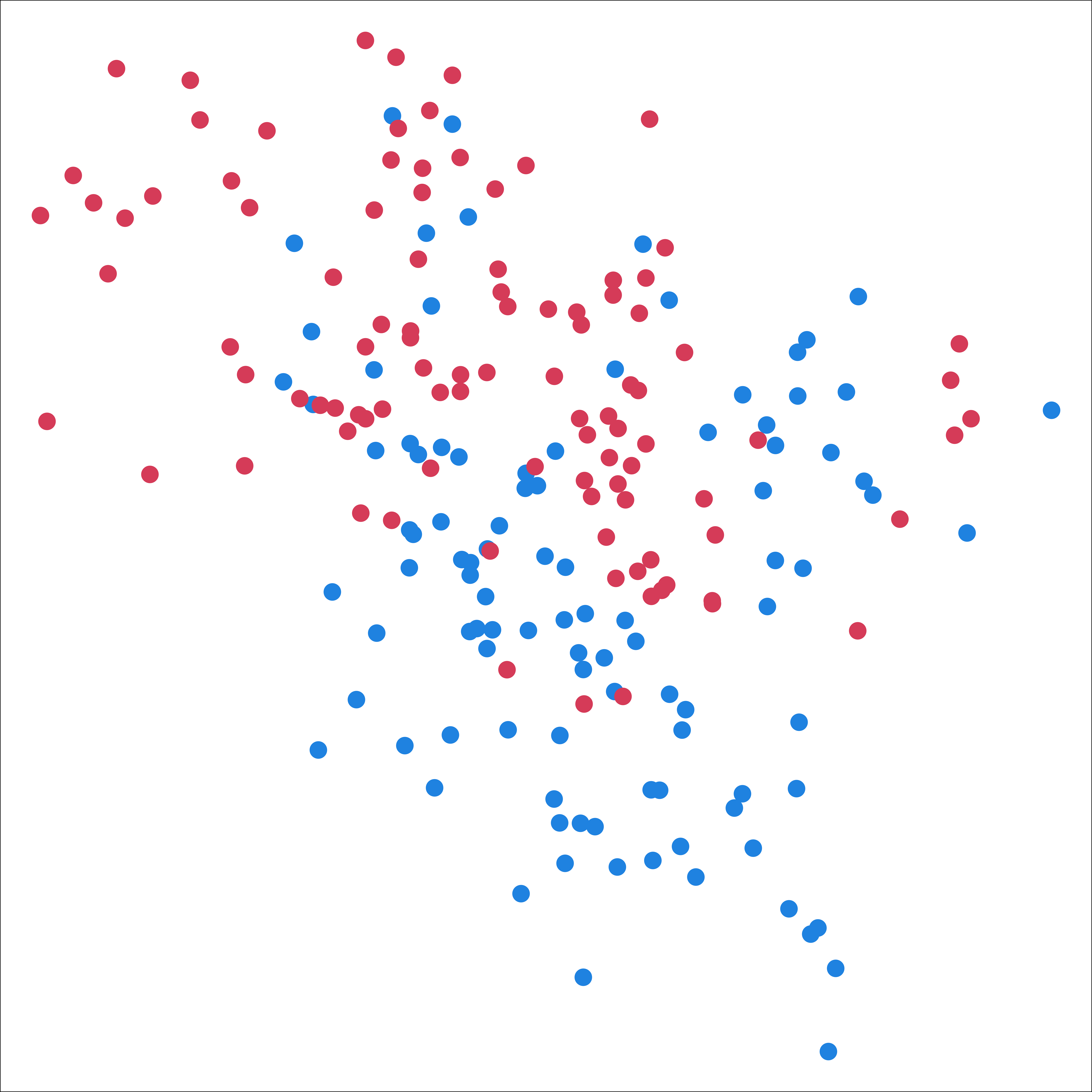
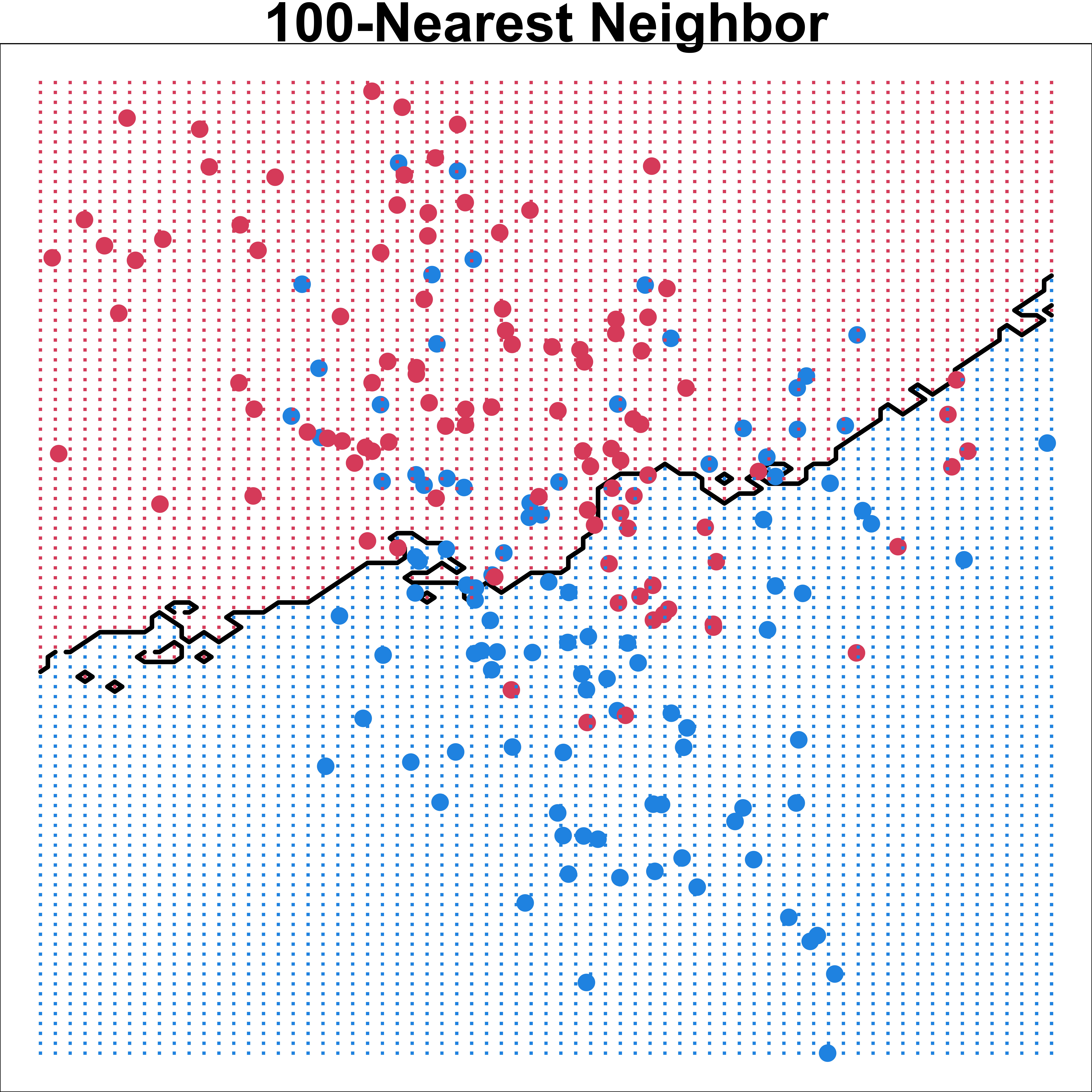
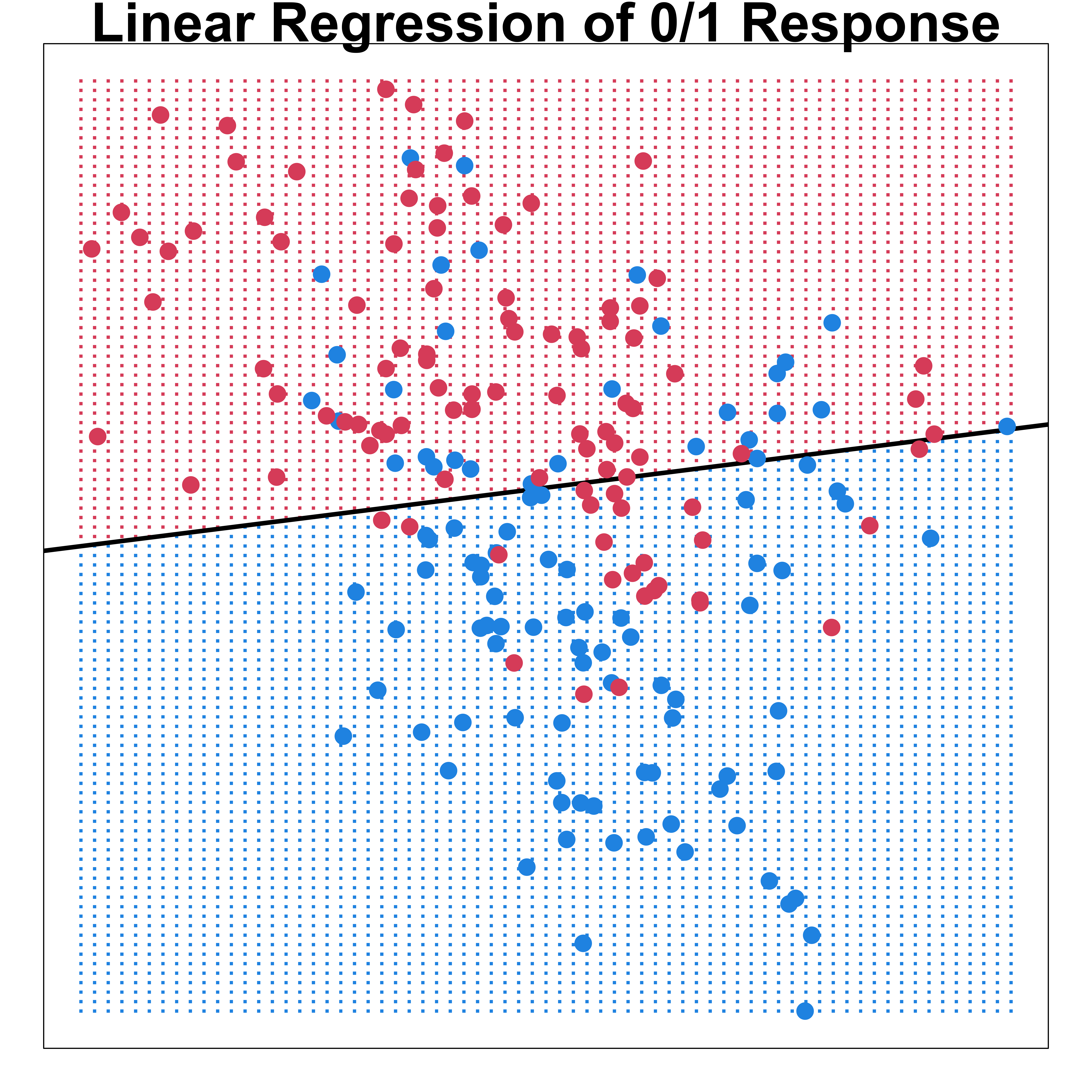
Example: ESL.mixture.rda

• The KNN decision boundary is nonlinear.

• R: class::knn(), kknn::kknn(), FNN::knn(), parsnip::nearest_neighbor()

• Python: from sklearn.neighbors import KNeighborsClassifier

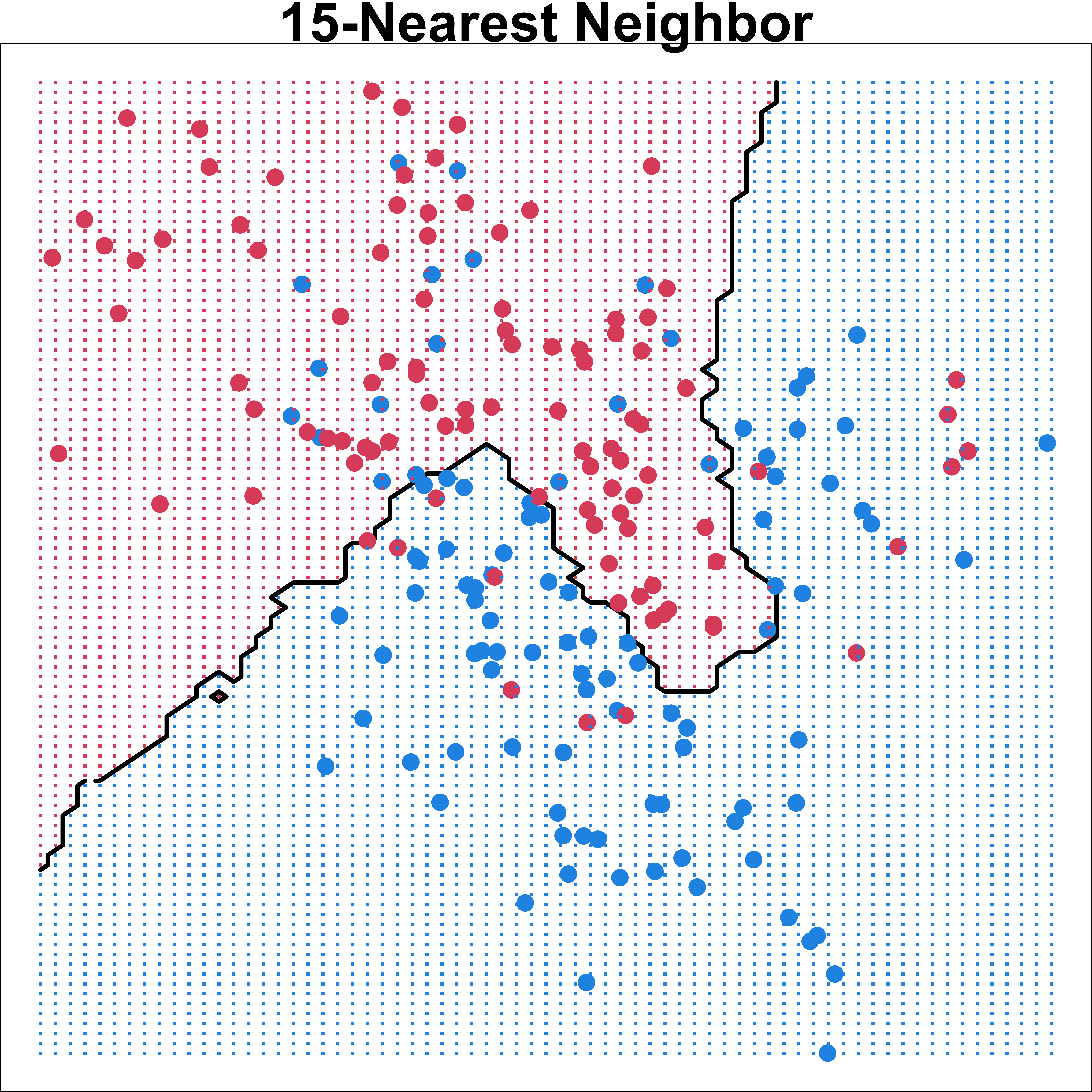
Example: ESL.mixture.rda

Confusion Matrix

  knn_fit <- class::knn(train = x, test = x, cl = y, k = 15)
  caret::confusionMatrix(table(knn_fit, y))

Confusion Matrix and Statistics

       y
knn_fit  0  1
      0 82 13
      1 18 87
                                        
               Accuracy : 0.845         
                 95% CI : (0.787, 0.892)
    No Information Rate : 0.5           
    P-Value [Acc > NIR] : <2e-16        
                                        
                  Kappa : 0.69          
                                        
 Mcnemar's Test P-Value : 0.472         
                                        
            Sensitivity : 0.820         
            Specificity : 0.870         
         Pos Pred Value : 0.863         
         Neg Pred Value : 0.829         
             Prevalence : 0.500         
         Detection Rate : 0.410         
   Detection Prevalence : 0.475         
      Balanced Accuracy : 0.845         
                                        
       'Positive' Class : 0             
                                        

Choosing K

set.seed(2024)
library(caret)
control <- trainControl(method = "cv", number = 10)
knn_cvfit <- train(y ~ ., method = "knn", 
                   data = data.frame("x" = x, "y" = as.factor(y)),
                   tuneGrid = data.frame(k = seq(1, 40, 1)),
                   trControl = control)
par(mar = c(4, 4, 0, 0))
plot(knn_cvfit$results$k, 1 - knn_cvfit$results$Accuracy,
     xlab = "K", ylab = "Classification Error", type = "b",
     pch = 19, col = 2)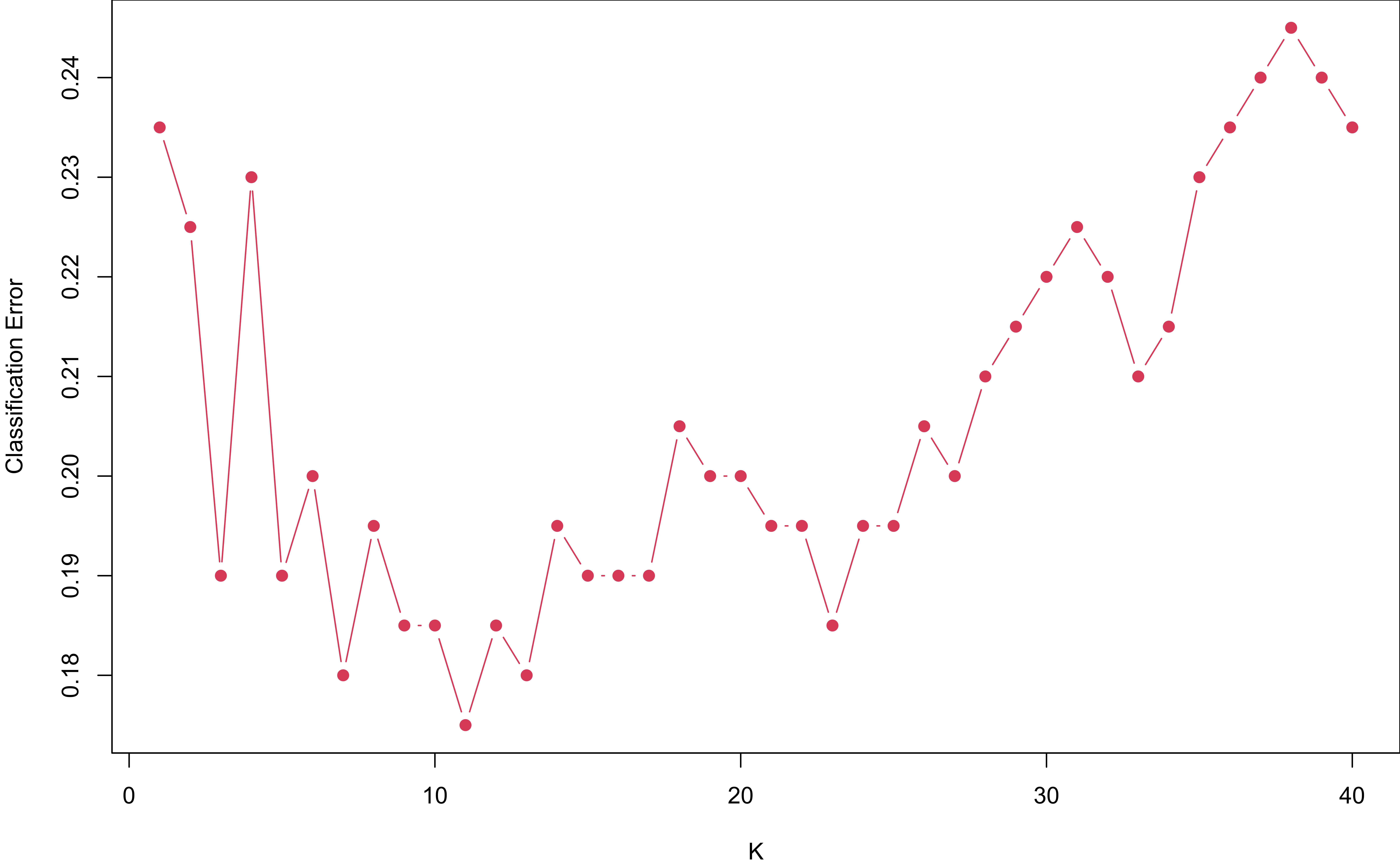

Scaling and Distance Measures

• By default, we use Euclidean distance (\(\ell_2\) norm).

\[d^2(\mathbf{u}, \mathbf{v}) = \lVert \mathbf{u}- \mathbf{v}\rVert_2^2 = \sum_{j=1}^p (u_j - v_j)^2\]

• This measure is not scale invariant: Multiplying the data with a factor changes the distance!

• Often consider a normalized version:

\[d^2(\mathbf{u}, \mathbf{v}) = \sum_{j=1}^p \frac{(u_j - v_j)^2}{\sigma_j^2}\]

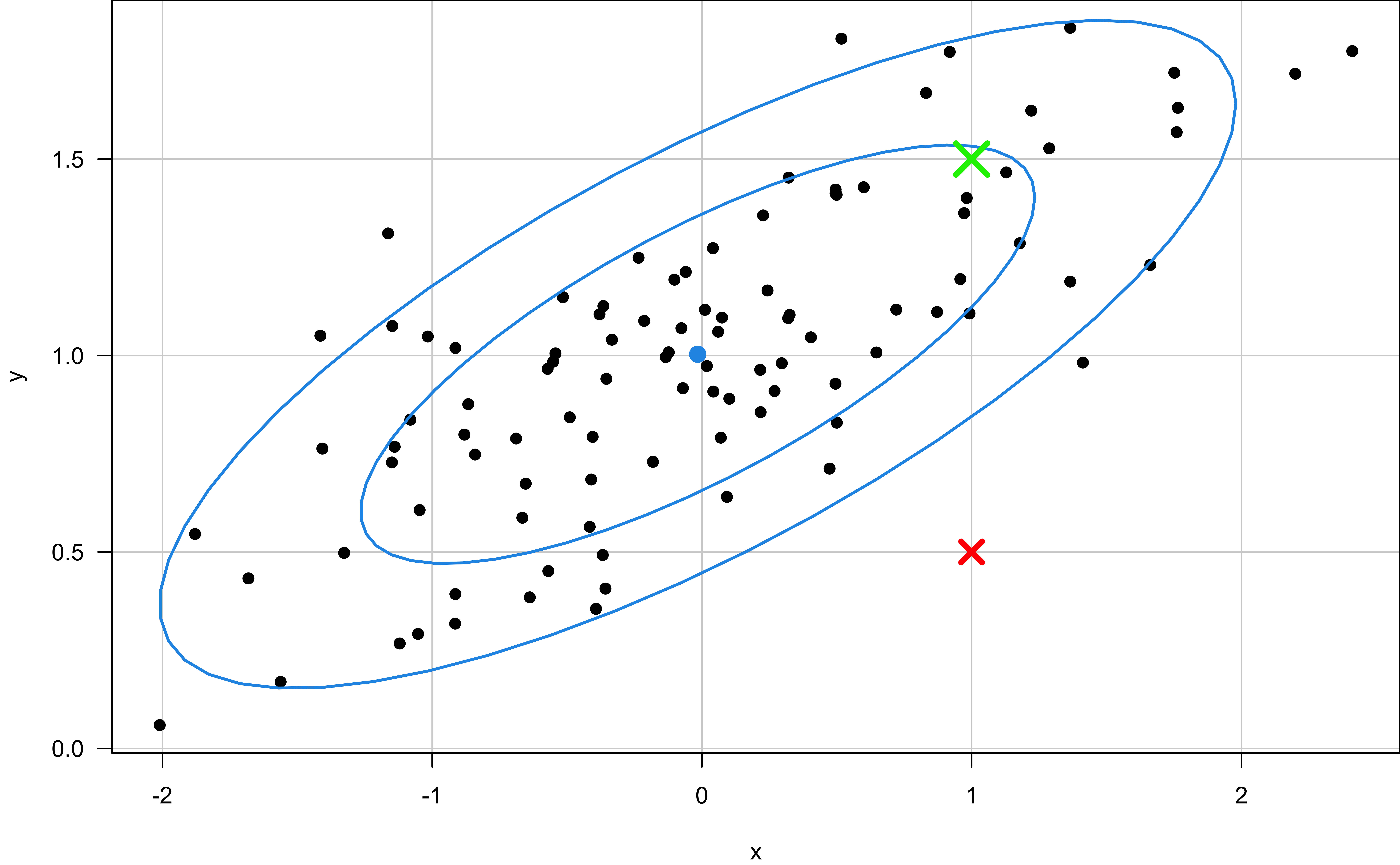
• Mahalanobis distance takes the covariance structure into account

\[d^2(\mathbf{u}, \mathbf{v}) = (\mathbf{u}- \mathbf{v})' \Sigma^{-1} (\mathbf{u}- \mathbf{v}),\]

• If \(\Sigma = \mathbf{I}\), Mahalanobis = Euclidean
• If \(\Sigma = diag(\sigma^2_1, \dots, \sigma^2_p)\), Mahalanobis = normalized version

Mahalanobis distance

• Red and green points have the same Euclidean distance to the center.

• The red point is farther away from the center in terms of Mahalanobis distance.

In the following plot, the red cross and orange cross have the same Euclidean distance to the center. However, the red cross is more of a “outlier” based on the joint distribution. The Mahalanobis distance would reflect this.

Example: Image Data ElemStatLearn::zip.train

• Digits 0-9 scanned from envelopes by the U.S. Postal Service

• \(16 \times 16\) pixel images, totally \(p=256\) variables

• At each pixel, we have the gray scale as the numerical value

• 1NN with Euclidean distance gives 5.6% error rate

• 1NN with tangent distance (Simard et al., 1993) gives 2.6% error

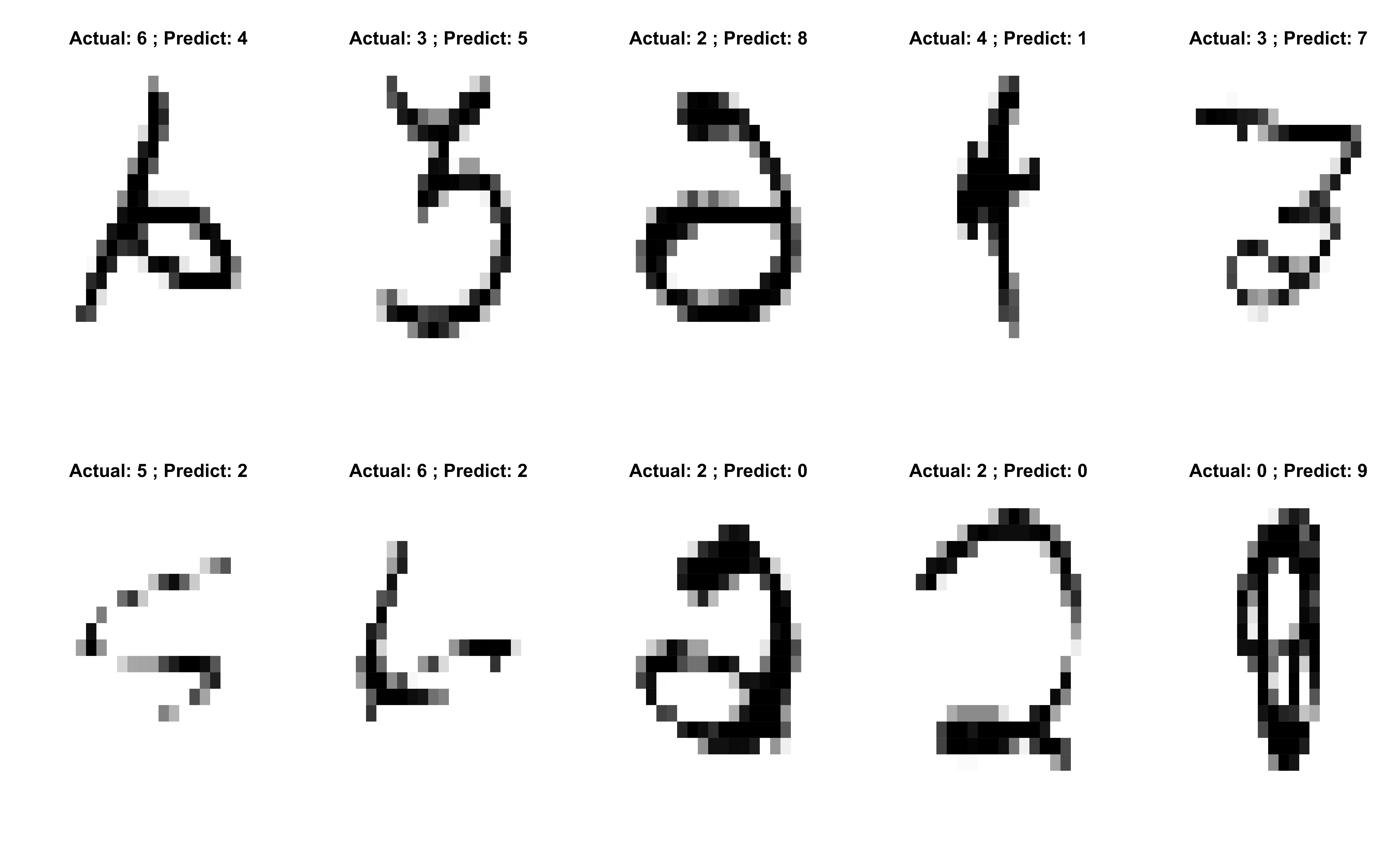
Example: 3NN on Image Data

  # fit 3nn model and calculate the error
  knn.fit <- class::knn(zip.train[, 2:257], zip.test[, 2:257], zip.train[, 1], k = 3)
  # overall prediction error
  mean(knn.fit != zip.test[, 1])

[1] 0.0533

  # the confusion matrix
  table(knn.fit, zip.test[, 1])

       
knn.fit   0   1   2   3   4   5   6   7   8   9
      0 355   0   7   2   0   3   3   0   4   2
      1   0 257   0   0   2   0   0   1   0   0
      2   2   0 183   2   0   2   1   1   0   0
      3   0   0   1 154   0   4   0   1   3   0
      4   0   3   1   0 183   0   2   4   0   3
      5   1   0   0   6   2 145   0   0   2   0
      6   0   2   0   0   2   1 164   0   0   0
      7   0   2   2   1   2   0   0 138   1   4
      8   0   0   4   0   1   1   0   1 153   0
      9   1   0   0   1   8   4   0   1   3 168

Example: 3NN on Image Data

Computational Issues

• Need to store the entire training data for prediction. (Lazy learner)

• Needs to calculate the distance from \(x_0\) to all training sample and sort them.¹

• Distance measures may affect accuracy.

\(K\)NN can be quite computationally intense for large sample size because to find the nearest neighbors, we need to calculate and compare the distances to each of the data point. In addition, it is not memory friendly because we need to store the entire training dataset for future prediction. In contrast, for linear model, we only need to store the estimated \(\boldsymbol \beta\) parameters. Some algorithms have been developed to search for the neighbors more efficiently. You can try the FNN package for these faster computations when \(n\) is large.

1. R FNN package for faster computations when \(n\) is large.

Curse of Dimensionality

• KNN does does not work well in high-dimensional space (\(p \gg n\)) due to curse of dimensionality.

As \(p\) increases, it’s getting harder to find \(k\) neighbors in the input space. KNN needs to explore a large range of values along each input dimension to grab the “neighbors”.

• The “neighbors” of \(x_0\) are in fact far away from \(x_0\), and so they may not be good predictors about the behavior of the function at \(x_0\).

• The method is not local anymore despite the name “nearest neighbor”!

• In high dimensions KNN often performs worse than linear regression.