Gaussian Processes ♾️

MSSC 6250 Statistical Machine Learning

Dr. Cheng-Han Yu
Department of Mathematical and Statistical Sciences
Marquette University

Gaussian Variables

Univariate Guassian

$Y \sim N(\mu, \sigma^2)$

Multivariate Guassian

“Multivariate” $=$ two or more random variables
$\mathbf{Y}\in \mathbb{R}^d \sim N_d\left(\boldsymbol \mu, \boldsymbol \Sigma\right)$

Bivariate Gaussian ($d=2$):

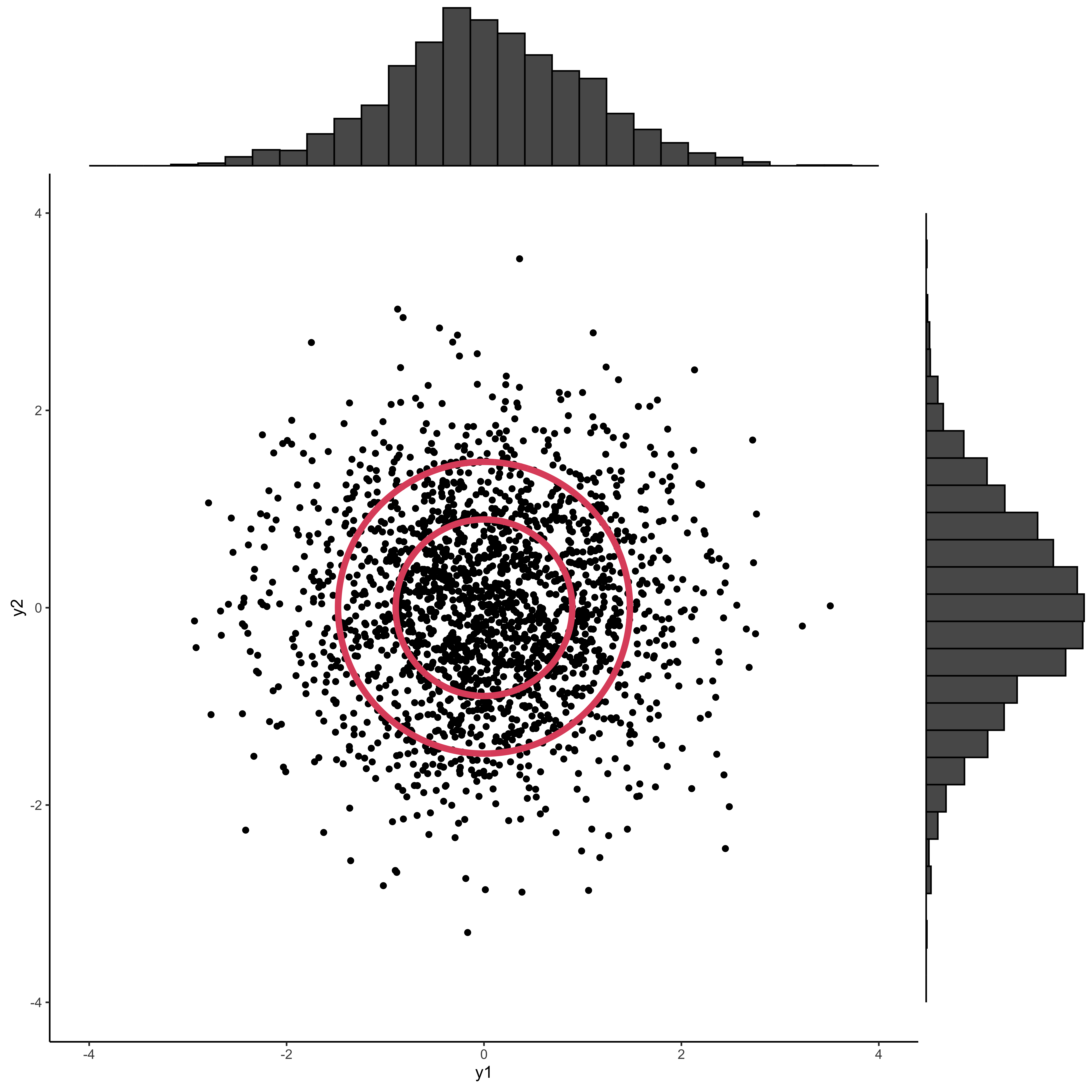
\[\mathbf{Y}= \begin{pmatrix} Y_1 \\ Y_2 \end{pmatrix}\] \[\boldsymbol \mu= \begin{pmatrix} \mu_1 \\ \mu_2 \end{pmatrix}\] \[\boldsymbol \Sigma= \begin{pmatrix} \sigma_1^2 & \rho_{12}\sigma_1\sigma_2\\ \rho_{12}\sigma_1\sigma_2 & \sigma_2^2 \end{pmatrix}\]

\[\boldsymbol \mu= \begin{pmatrix} 0 \\ 0 \end{pmatrix}\] \[\boldsymbol \Sigma= \begin{pmatrix}1 & 0\\ 0 & 1 \end{pmatrix}\]

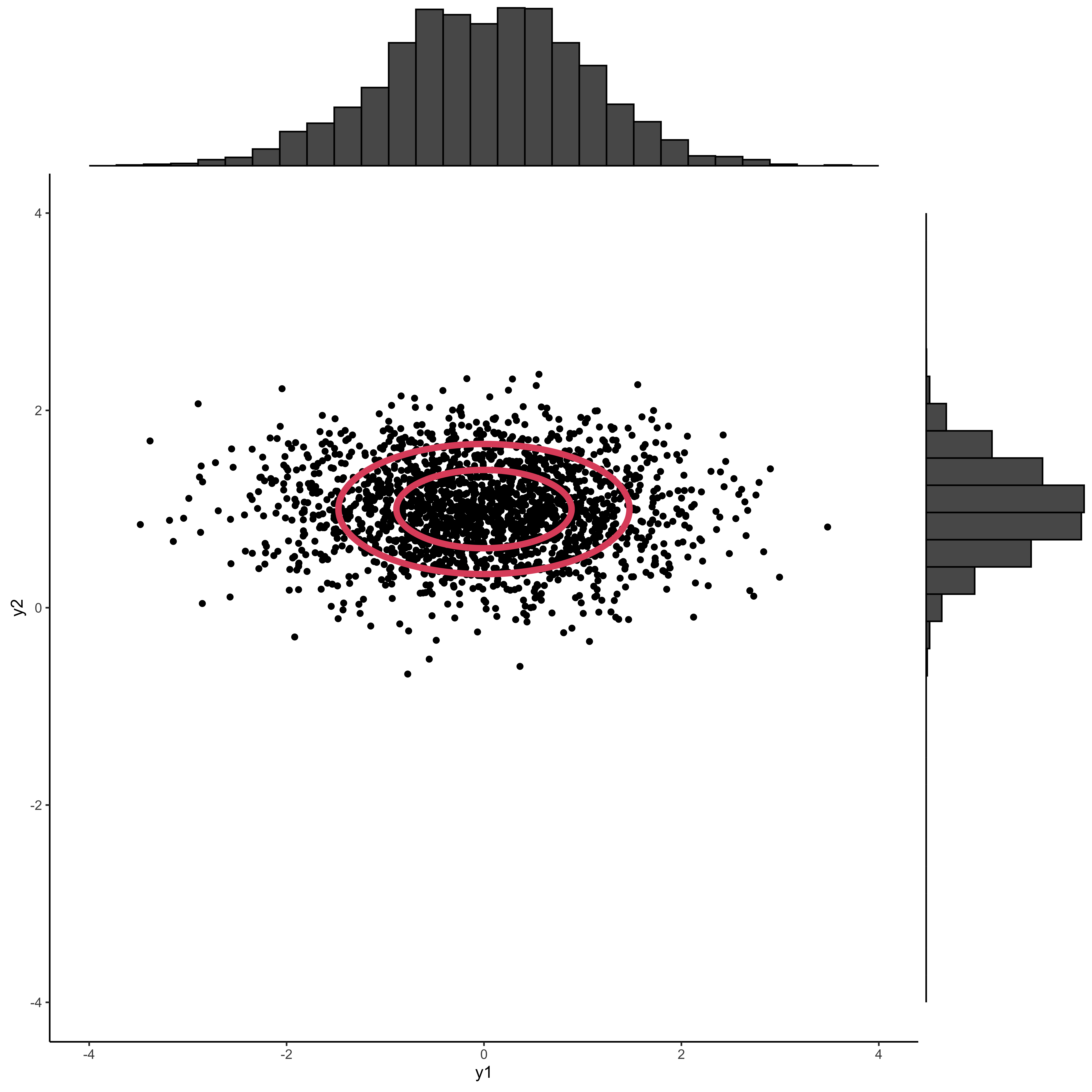
\[\boldsymbol \mu= \begin{pmatrix} 0 \\ 1 \end{pmatrix}\] \[\boldsymbol \Sigma= \begin{pmatrix}1 & 0\\ 0 & 0.2 \end{pmatrix}\]

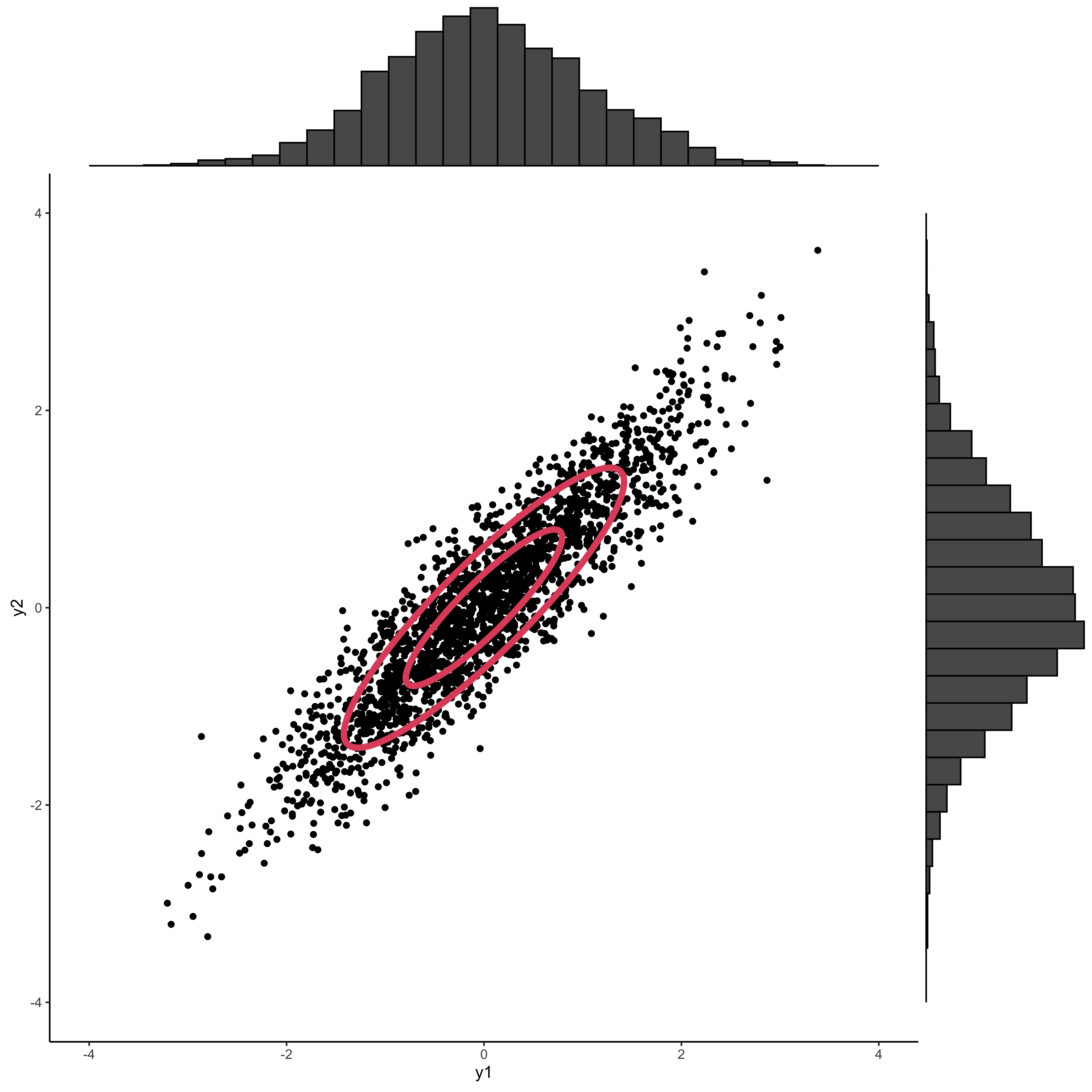
\[\boldsymbol \mu= \begin{pmatrix} 0 \\ 0 \end{pmatrix}\] \[\boldsymbol \Sigma= \begin{pmatrix}1 & 0.9\\ 0.9 & 1 \end{pmatrix}\]

Three or More Variables

Hard to visualize in dimensions $> 2$, so stack points next to each other.

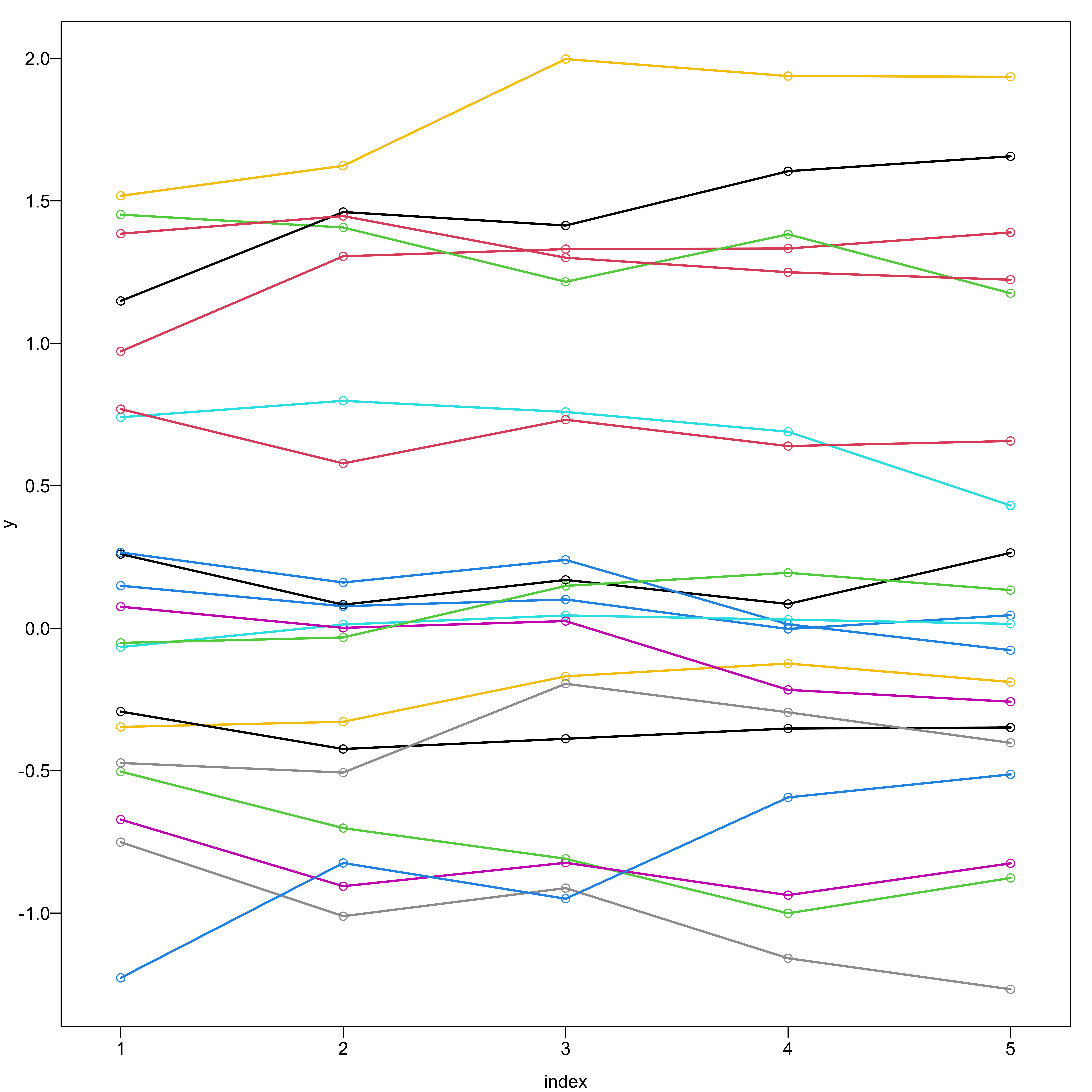
$d = 5$

\[\boldsymbol \mu= \begin{pmatrix} 0 \\ 0 \\ 0\\0\\0\end{pmatrix} \quad \quad \boldsymbol \Sigma= \begin{pmatrix}1 & 0.99 & 0.98 & 0.97 & 0.96\\ 0.99 & 1 & 0.99 & 0.98 & 0.97 \\ 0.98 & 0.99 & 1 & 0.99 & 0.98 \\ 0.97 & 0.98 & 0.97 & 1 & 0.99\\0.96 & 0.97 & 0.98 & 0.99 & 1 \end{pmatrix}\]

Each line is one sample (path).

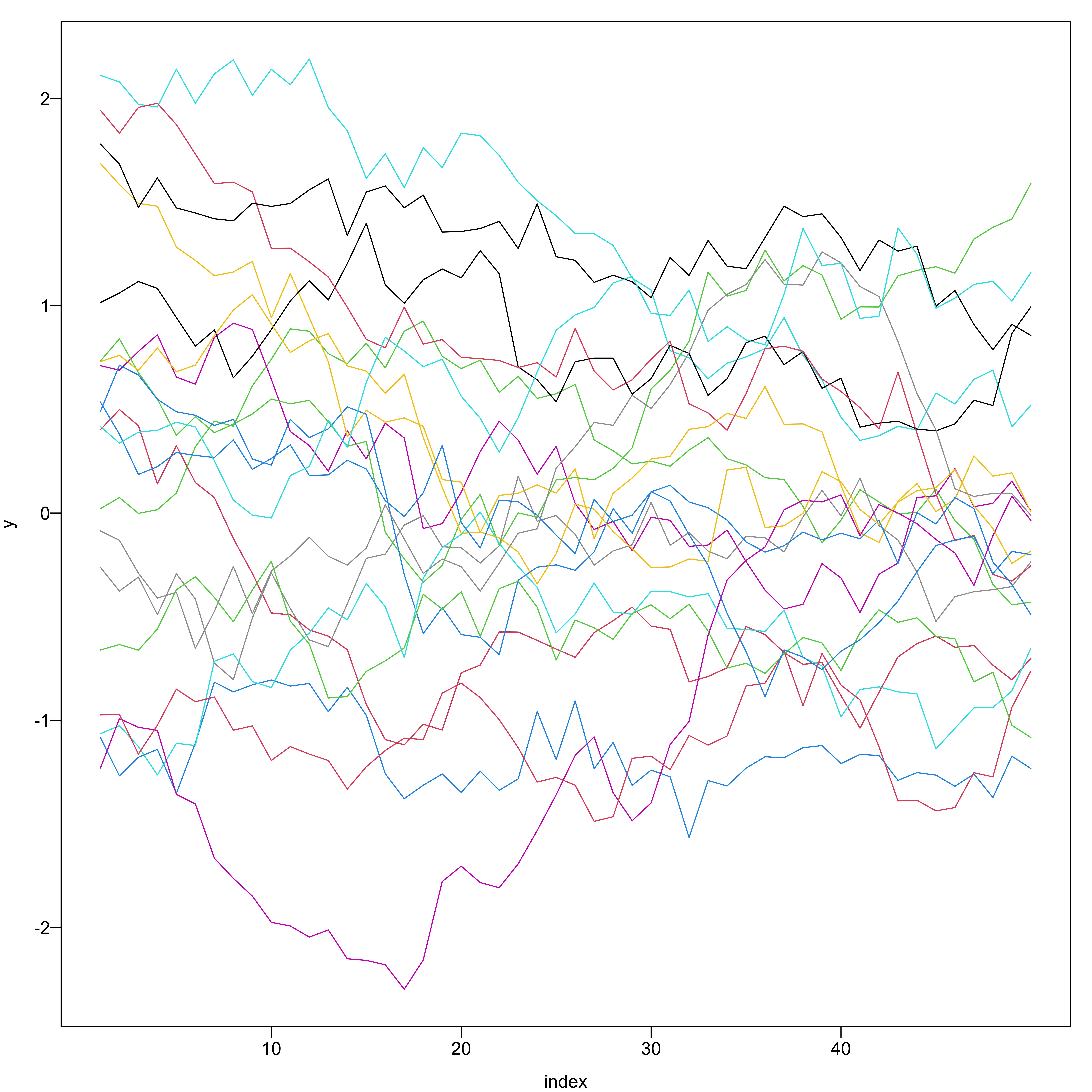
$d = 50$

\[\boldsymbol \mu= \begin{pmatrix} 0 \\ 0 \\ \vdots \\0\\0\end{pmatrix} \quad \quad \boldsymbol \Sigma= \begin{pmatrix} 1 & 0.99 & 0.98 & 0.97 & 0.96 & \cdots \\ 0.99 & 1 & 0.99 & 0.98 & 0.97 & \cdots\\ 0.98 & 0.99 & 1 & 0.99 & 0.98 & \cdots\\ 0.97 & 0.98 & 0.97 & 1 & 0.99 & \cdots\\ 0.96 & 0.97 & 0.98 & 0.99 & 1 & \cdots \\ \vdots & \vdots & \vdots & \vdots & \vdots & \vdots & \end{pmatrix}\]

Each line is one sample (path).
Think of Gaussian processes as an infinite dimensional distribution over functions
- all we need to do is change notation

Gaussian Processes

A stochastic process $f(x), x \in \mathcal{X} \subset \mathbb{R}^D$, is a function whose values are random variables, for any value of $x$.
Usually for $D = 1$, the process is a temporal process, and for $D > 1$, it is referred to as a spatial process.

A Gaussian process (GP) is a process where all finite-dimensional distributions are multivariate Gaussian, for any choice of $n$ and $x_1\dots, x_n \in \mathbb{R}^D$:

\[f(x_1), \dots, f(x_n) \sim N_n\left(\boldsymbol \mu, \boldsymbol \Sigma\right)\]

Write $Y(\cdot) \sim GP$ to denote that the function $Y$ is a GP.

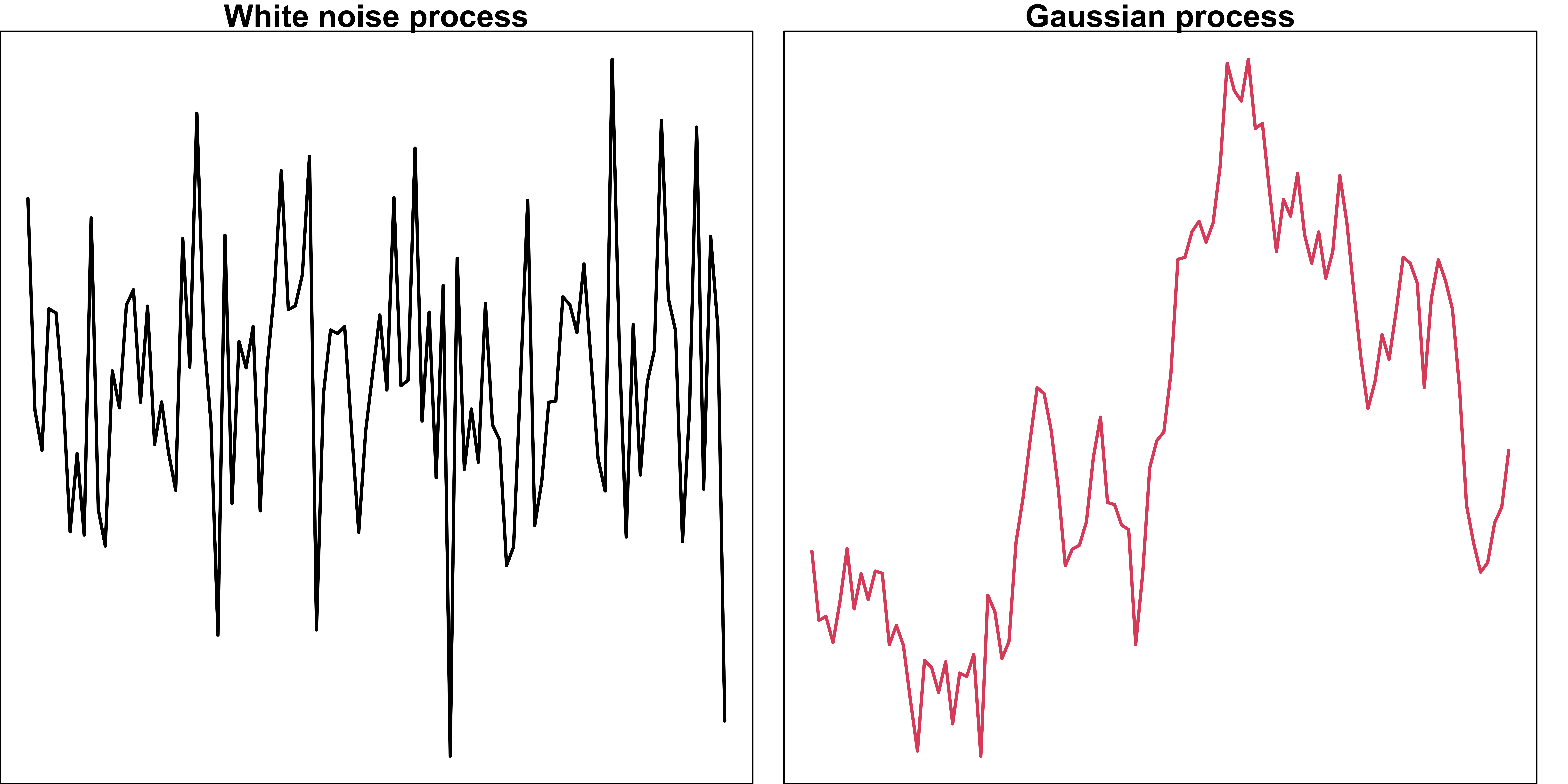
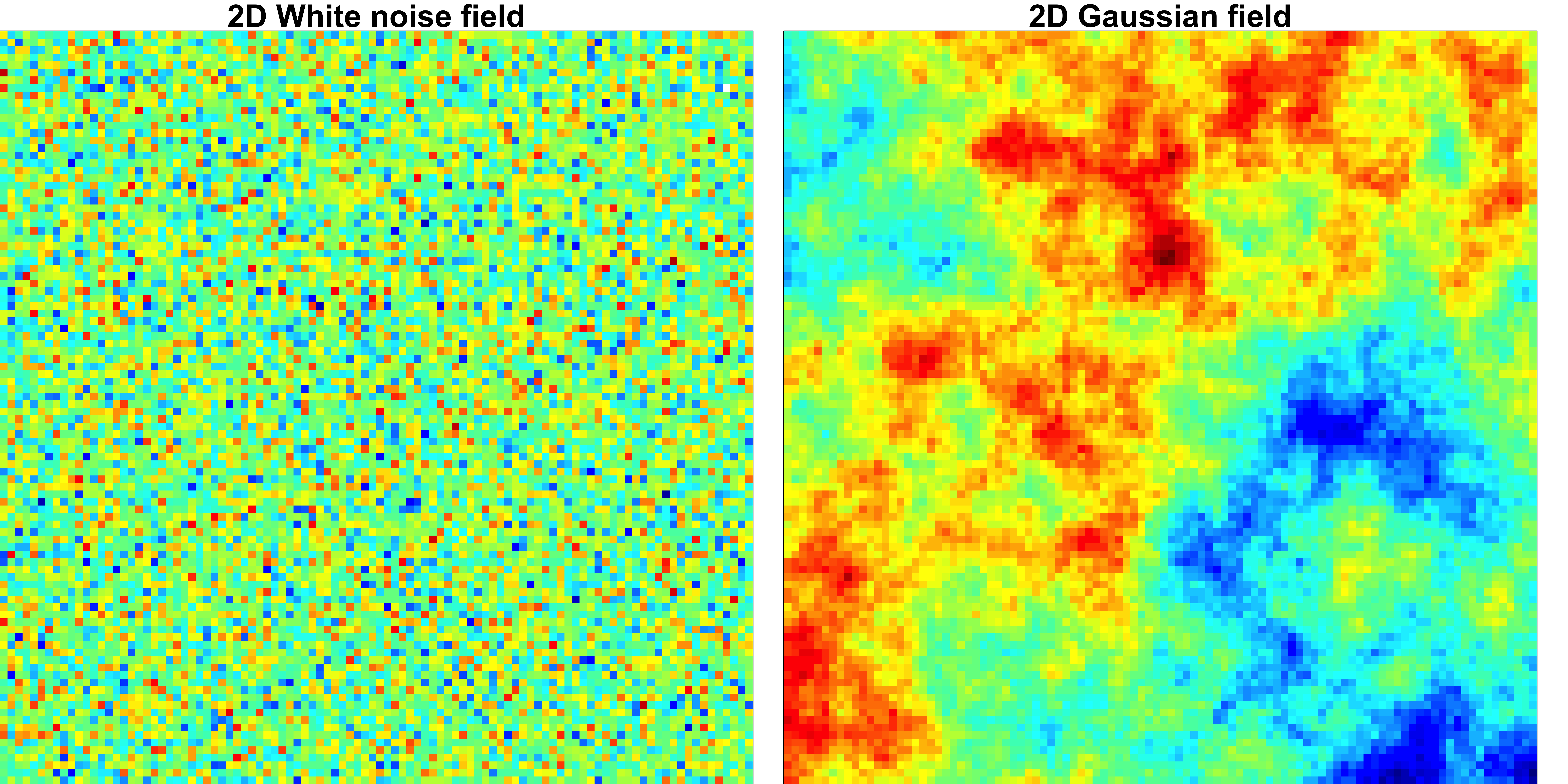
Mean and Covariance Function

To fully specify a Gaussian distribution we need the mean and covariance, $Y \sim N(\mu, \Sigma)$

To fully specify a Gaussian process we need the mean and covariance function, \[f(\cdot) \sim GP\left(m(\cdot), k(\cdot, \cdot)\right)\] where

\[\text{E}(f(x)) = m(x)\] \[\text{Cov}(f(x), f(x')) = k(x, x')\]

Popular choices of $m(\cdot)$ are $m(x) = 0$ or $m(x) = \text{const}$ for all $x$, or $m(x) = \beta'x$
Care more about the covariance function or kernel function as it governs the how the process looks like by defining the similarity between data points.

Covariance Function Kernel

\[\text{Cov}(f(x), f(x')) = k(x, x')\]

$k(x, x')$ must be a positive semi-definite function, leading to valid covariance matrices:
- Given locations $x_1, \dots, x_n$, the $n \times n$ Gram matrix $K$ with $K_{ij} = k(x_i, x_j)$ must be a positive semi-definite matrix.

Often assume $k(x, x')$ is a function of only the distance between locations: \[\text{Cov}(f(x), f(x')) = k(\|x-x'\|) = k(r)\]
- the GP is a stationary process.
- the covariance function is isotropic.

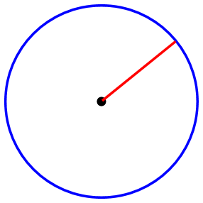
The covariance function determines the nature of the GP, hypothesis space of functions.

Squared Exponential (SE) Kernel

\[k(x, x' \mid \tau, h) = \tau^2 \exp\left(-\frac{(x - x')^2}{2h^2} \right)\]

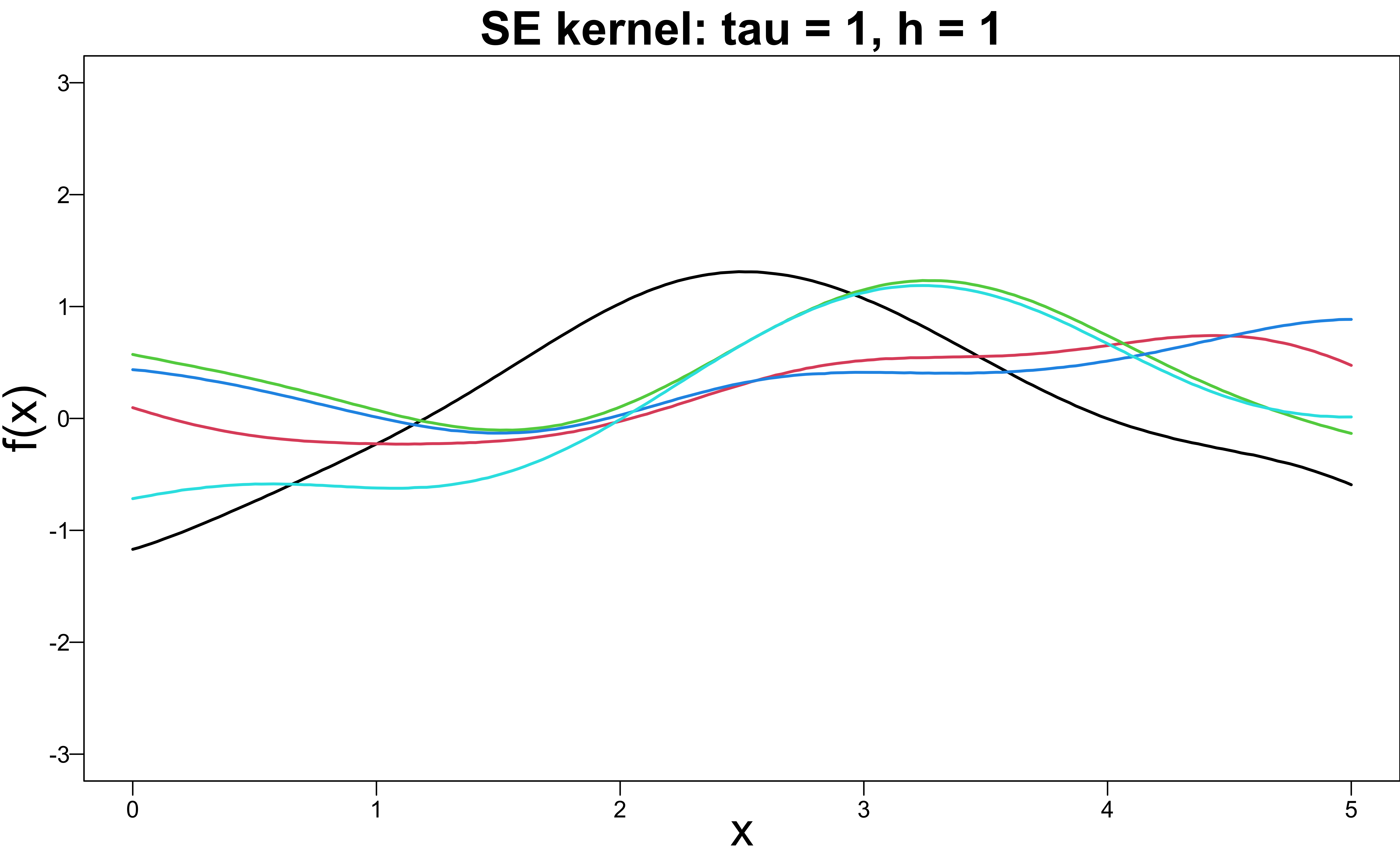
\[k(x, x') = \exp\left(-\frac{1}{2}(x - x')^2 \right)\]

Squared Exponential (SE) Kernel

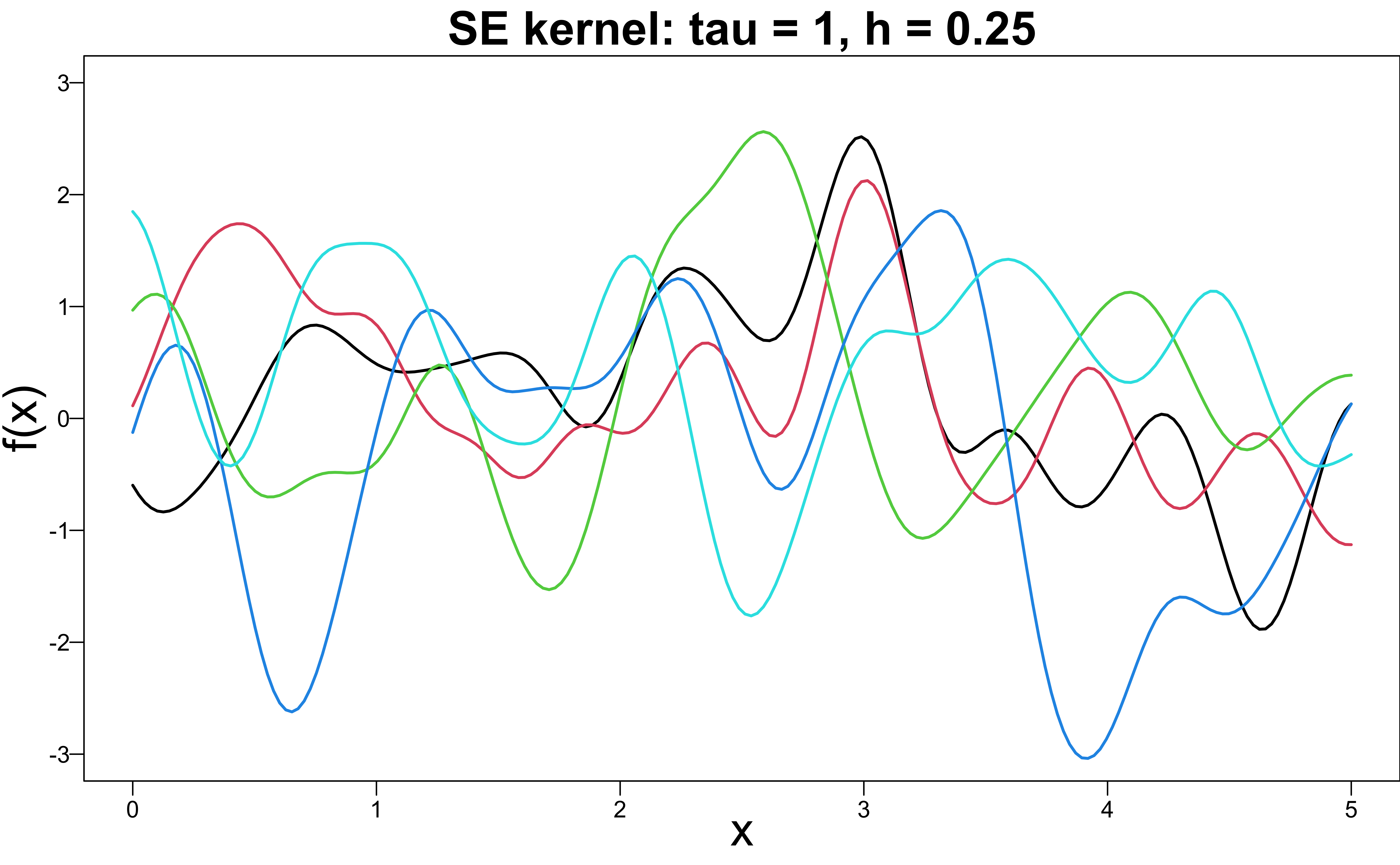
\[k(x, x') = \exp\left(-\frac{1}{2}\frac{(x - x')^2}{ {\color{red}{0.25}}^2} \right)\]

The parameter $h$ is the characteristic length-scale that controls the number of level-zero upcrossings.

Squared Exponential (SE) Kernel

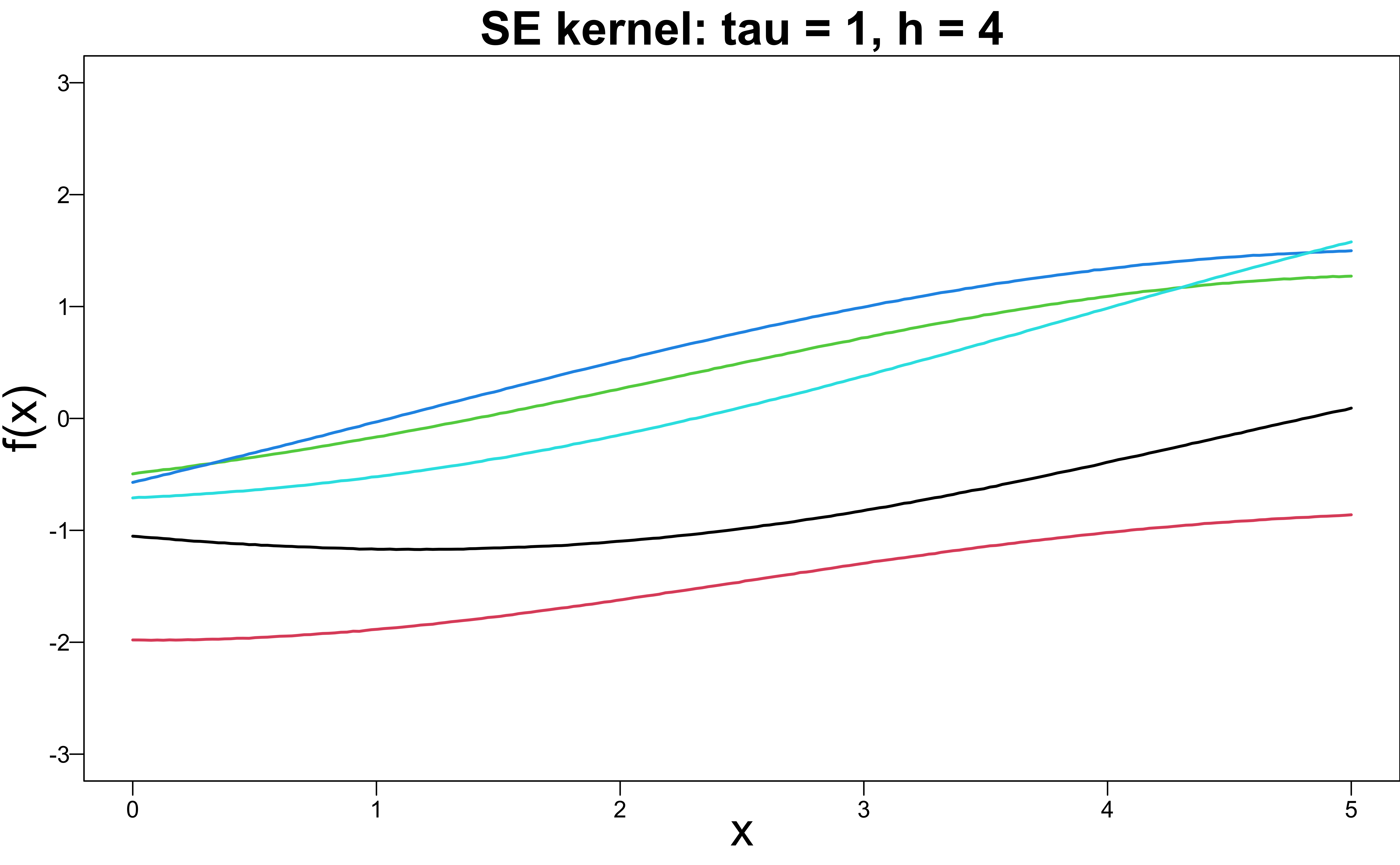
\[k(x, x') = \exp\left(-\frac{1}{2}\frac{(x - x')^2}{ {\color{red}{4}}^2} \right)\]

Squared Exponential (SE) Kernel

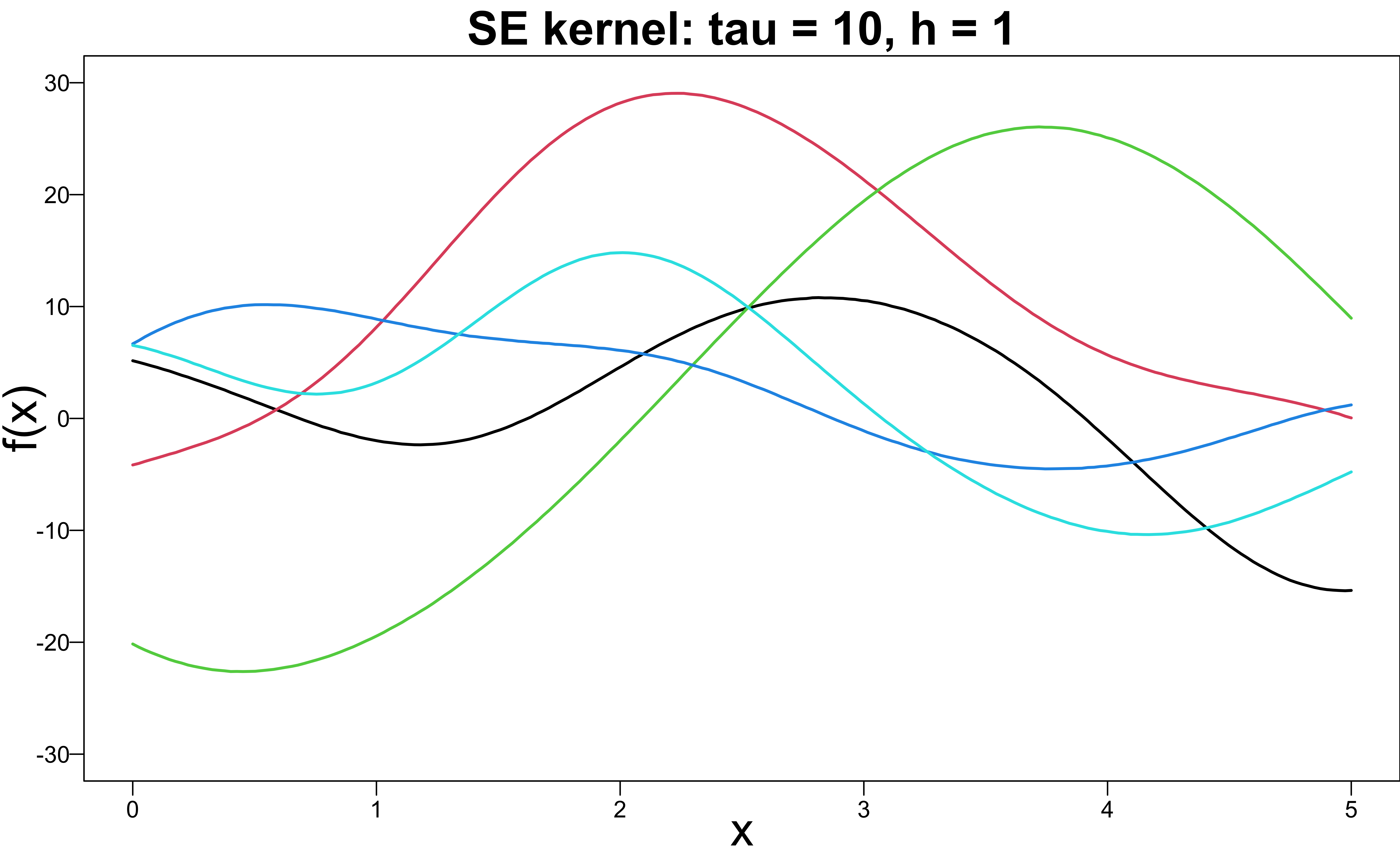
\[k(x, x') = {\color{red}{10^2}}\exp\left(-\frac{1}{2}(x - x')^2 \right)\]

The parameter $\tau$ is the variance of $f(x)$ that controls the vertical variation of the process.

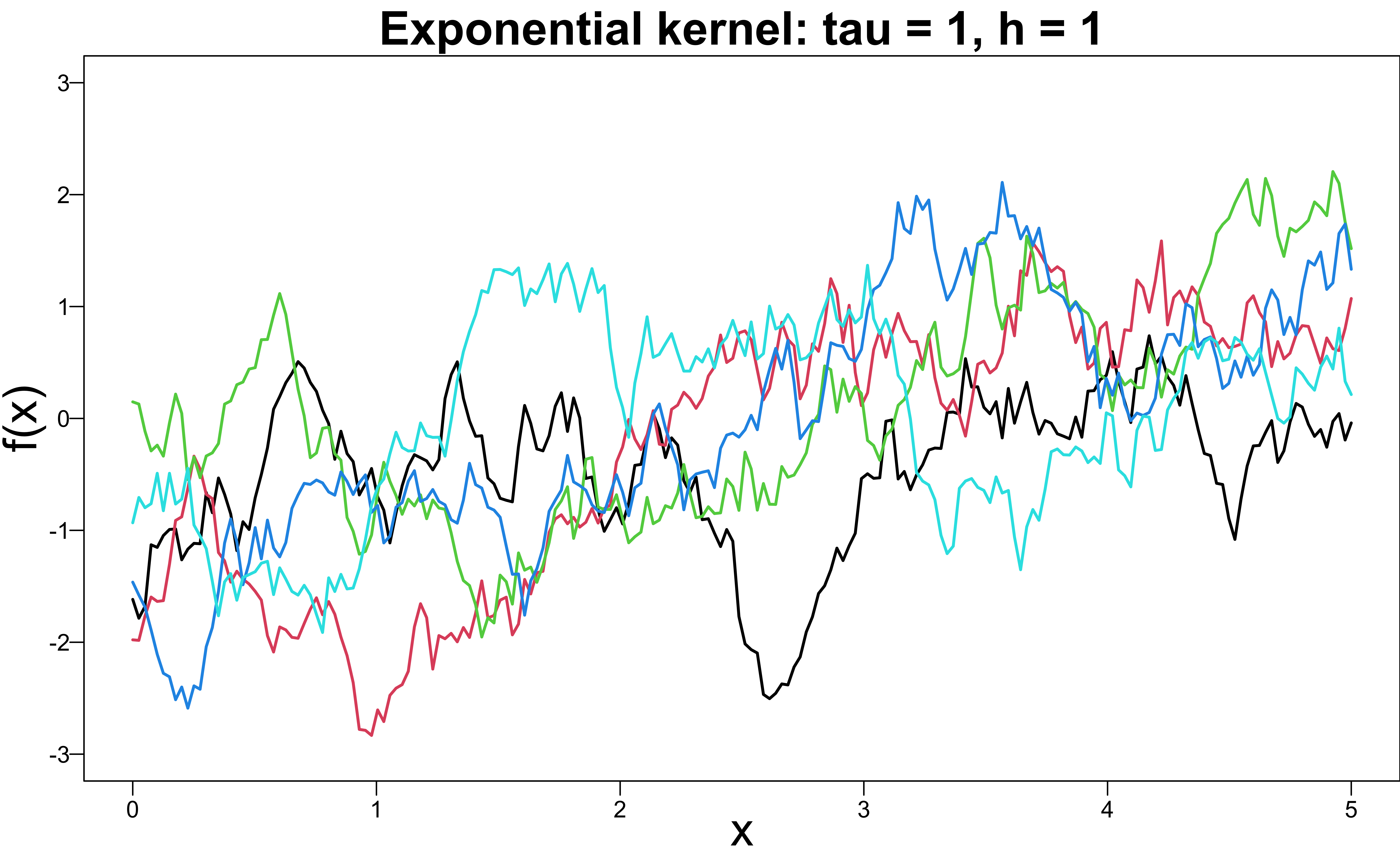
Exponential Kernel

\[k(x, x' \mid \tau, h) = \tau^2 \exp\left(-\frac{|x - x'|}{h} \right)\]

Brownian Motion

\[k(x, x') = \min(x, x')\]

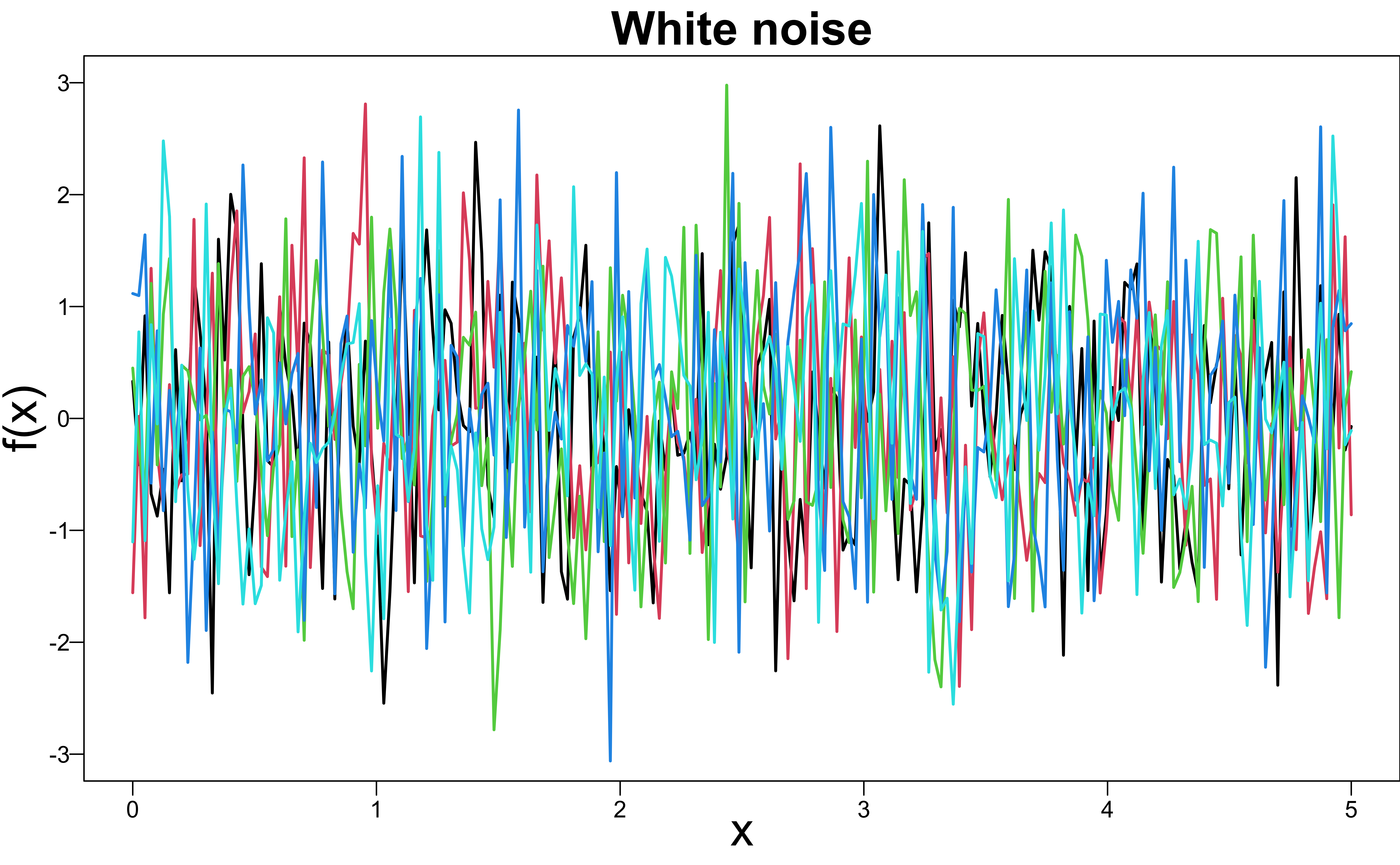
White Noise

\[k(x, x') = \begin{cases} 1 & \quad \text{if } x = x' \\ 0 & \quad \text{otherwise} \end{cases}\]

Why GP?

The GP inherits its properties primarily from the covariance function $k$:
- Smoothness
- Differentiability
- Variance

Sums of Gaussians are Gaussian.

Marginal distributions of multivariate Gaussians are still Gaussian.

Any affine transformation of a Gaussian is a Gaussian.

Conditional distributions are still Gaussian.

\[\mathbf{Y}= \begin{pmatrix} \mathbf{Y}_1 \\ \mathbf{Y}_2 \end{pmatrix} \sim N\left(\boldsymbol \mu, \boldsymbol \Sigma\right), \quad \boldsymbol \mu= \begin{pmatrix} \boldsymbol \mu_1 \\ \boldsymbol \mu_2 \end{pmatrix}, \quad \boldsymbol \Sigma= \begin{pmatrix} \Sigma_{11} & \Sigma_{12}\\ \Sigma_{21} & \Sigma_{22} \end{pmatrix}\] \[(\mathbf{Y}_2 \mid \mathbf{y}_1 = \mathbf{y}_1) \sim N\left(\boldsymbol \mu_2 + \Sigma_{21} \Sigma_{11}^{-1} (\mathbf{y}_1 - \boldsymbol \mu_1), \Sigma_{22} - \Sigma_{21}\Sigma_{11}^{-1}\Sigma_{12}\right)\]

Conditional Updates of Gaussian Processes

If $f(\cdot) \sim GP$,

\[f(x_1), \dots, f(x_n), f(x) \sim N(\boldsymbol \mu, \boldsymbol \Sigma)\]

If we observe its value at $x_1, \dots, x_n$, then

\[f(x) \mid f(x_1), \dots, f(x_n) \sim N(\boldsymbol \mu^*, \boldsymbol \Sigma^*)\] where $\boldsymbol \mu^*$ and $\boldsymbol \Sigma^*$ are as on the previous slide.

We still believe $f$ is a GP even we’ve observed its value at a number of locations.

Gaussian Process Regression

Bayesian Conditioning Updates of GP: Prior

Instead of assigning priors to parameters in the regression function, we assign a function prior to the regression function:

\[f(\cdot) \sim GP(0, k(\cdot, \cdot))\]

For any points $x_1, \dots, x_n, x^*$,

\[f(x_1), \dots, f(x_n), f(x^*) \sim N\left(0, \boldsymbol \Sigma\right)\]

\[\boldsymbol \Sigma= \left(\begin{array}{ccc|c} k(x_1, x_1) & \cdots & k(x_1, x_n) & k(x_1, x^*) \\ \vdots & & \vdots & \vdots \\ k(x_n, x_1) & \cdots & k(x_n, x_n) & k(x_n, x^*) \\ \hline k(x^*, x_1) & \cdots & k(x^*, x_n) & k(x^*, x^*) \end{array} \right) = \left(\begin{array}{ccc|c} & & & \\ & K & & K_* \\ & & & \\ \hline & K_*^T & & K_{**} \end{array} \right) \]

Bayesian Conditioning Updates of GP: Posterior

Given observed information $f(x_1), \dots, f(x_n)$

\[f(x^*) \mid f(x_1), \dots, f(x_n) \sim N\left( \boldsymbol \mu^*, \boldsymbol \Sigma^*\right)\] where

\[\boldsymbol \mu^* = K_{*}^TK^{-1}{\bf f}\] with ${\bf f} = \left(f(x_1), \dots, f(x_n)\right)^T$

\[\boldsymbol \Sigma^* = K_{**} - K_{*}^TK^{-1}K_{*}\]

No Noise/Nugget - Interpolation

—–: posterior mean $\boldsymbol \mu^*$
—–: 95% posterior predictive interval $\boldsymbol \mu^* \pm 1.96 \boldsymbol \Sigma^*$
So far we treat $f(x)$, the function values as data points.
There is no noise, and every posterior curve interpolates data points.

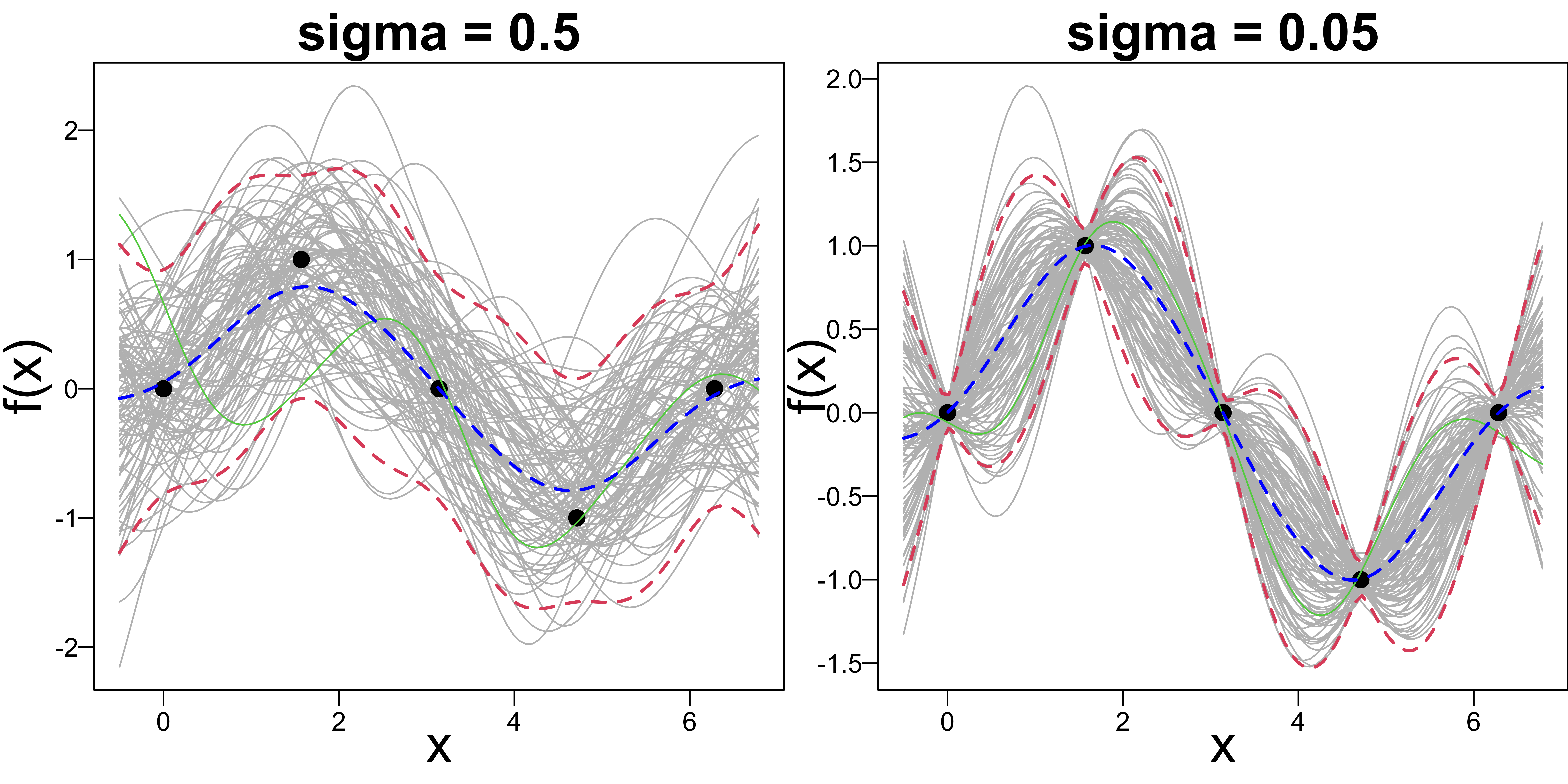
Noisy Observations/with Nugget - GP Regression (GPR)

In reality, we don’t or can’t observe $f(x)$ and like to estimate it.

\[\begin{align} y_i &= f(x_i) + \epsilon_i, \quad \epsilon_i\sim N(0, \sigma^2) \\ f(\cdot) &\sim GP(0, k(\cdot, \cdot; \theta))\end{align}\]

$$$$

\[y_1, \dots, y_n, f(x^*) \sim N\left(0, \boldsymbol \Sigma\right), \quad \boldsymbol \Sigma= \left(\begin{array}{ccc|c} & & & \\ & K + \sigma^2I & & K_* \\ & & & \\ \hline & K_*^T & & K_{**} \end{array} \right) \]

\[f(x^*) \mid y_1, \dots, y_n \sim N\left( \boldsymbol \mu^*, \boldsymbol \Sigma^*\right), \quad \boldsymbol \mu^* = K_{*}^T{\color{red}{(K + \sigma^2I)^{-1}}}{\bf y}, \quad \boldsymbol \Sigma^* = K_{**} - K_{*}^T{\color{red}{(K + \sigma^2I)^{-1}}}K_{*}\] with ${\bf y} = \left(y_1, \dots, y_n\right)^T$

Noisy Observations/with Nugget - GP Regression (GPR)

Hyperparameter Tuning

Empirical Bayes

Uses the observed data to estimate parameters $\theta = (\sigma^2, \tau^2, h)$
Find an empirical Bayes estimate for $\theta$ from the marginal likelihood

\[ p\left( \mathbf{y}\mid \theta \right) = \int p\left( \mathbf{y}\mid {\bf f} \right) p\left( {\bf f} \mid \theta \right) \, d {\bf f} = N\left(\mathbf{0}, K(\tau, h)+\sigma^2I \right)\]

$\hat{\theta}_{EB} = \mathop{\mathrm{arg\,max}}_{\theta}\log p\left( \mathbf{y}\mid \theta \right)$.

Full Bayesian Inference

\[\begin{align} y_i &= f(x_i) + \epsilon_i, \, \, \epsilon_i \stackrel{\rm iid}{\sim} N(0, \sigma^2), \quad i = 1, \dots, n,\\ f(\cdot) &\sim GP\left(\mu, k(\cdot, \cdot)\right),\,\, \text{Cov}(f(x_i), f(x_j)) = k(x_i, x_j)\\ \sigma^2 &\sim IG(a_{\sigma}, b_{\sigma})\\ \tau^2 &\sim IG(a_{\tau}, b_{\tau})\\ h &\sim Ga(a_{h}, b_{h})\\ \mu & \sim N(0, b_{\mu}) \end{align}\]

The model is Gibbsable, or the Metropolis-Hastings algorithm can be used when ${\bf f}$ is integrated out.

Gaussian Process Classification