Support Vector Machines

MSSC 6250 Statistical Machine Learning

Dr. Cheng-Han Yu
Department of Mathematical and Statistical Sciences
Marquette University

Support Vector Machines (SVMs)

• SVMs have been shown to perform well in a variety of settings, and are often considered one of the best “out of the box” classifiers.

• Start with the maximal margin classifier (1960s), then the support vector classifier (1990s), and then the support vector machine.

Classifier

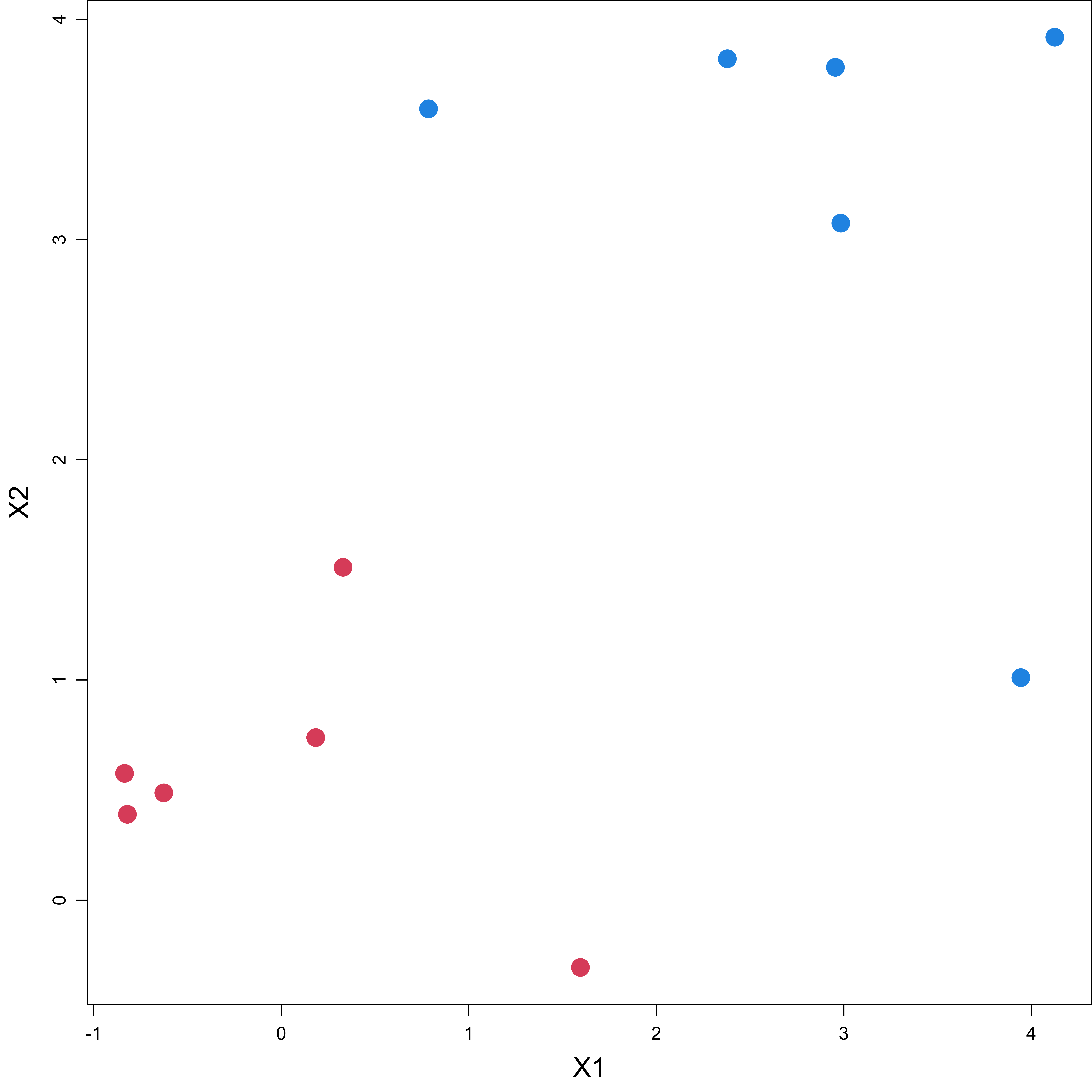
• \({\cal D}_n = \{\mathbf{x}_i, y_i\}_{i=1}^n\)

• In SVM, we code the binary outcome \(y\) as 1 or -1, representing one class and the other.

• The goal is to find a linear classifier \(f(\mathbf{x}) = \beta_0 + \mathbf{x}' \boldsymbol \beta\) so that the classification rule is the sign of \(f(\mathbf{x})\):

\[ \hat{y} = \begin{cases} +1, \quad \text{if} \quad f(\mathbf{x}) > 0\\ -1, \quad \text{if} \quad f(\mathbf{x}) < 0 \end{cases} \]

Separating Hyperplane

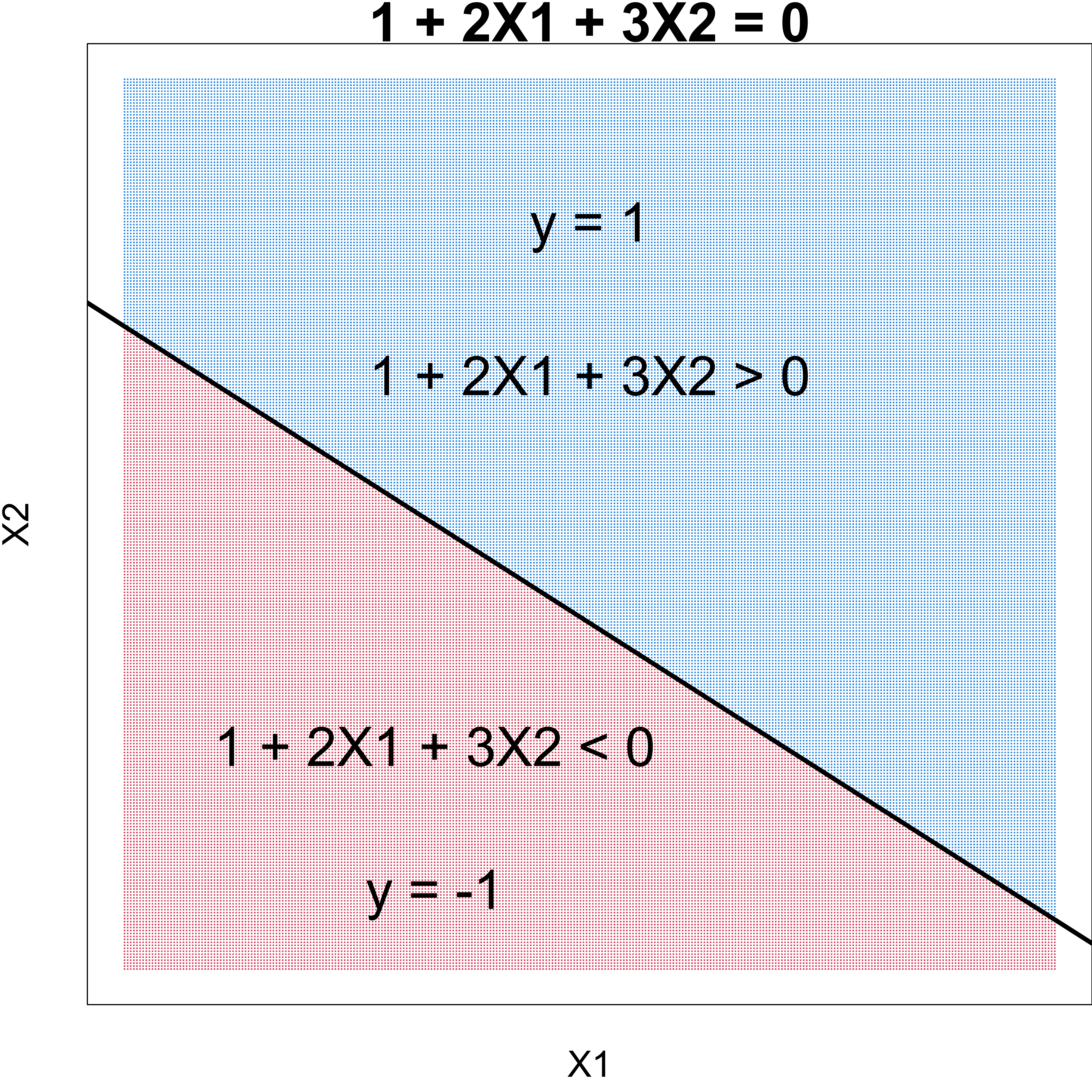
• The \(f(\mathbf{x}) = \beta_0 + \mathbf{x}' \boldsymbol \beta= 0\) is a hyperplane, which is a subspace of dimension \(p-1\) in the \(p\)-dimensional space.

• \(f(\mathbf{x}) = \beta_0 + \beta_1X_1+\beta_2X_2 = 0\) is a straight line (hyperplane of dimension one) in the 2-dimensional space.

• The classification rule is \(y_i f(\mathbf{x}_i) >0\).

Maximum-margin Classifier

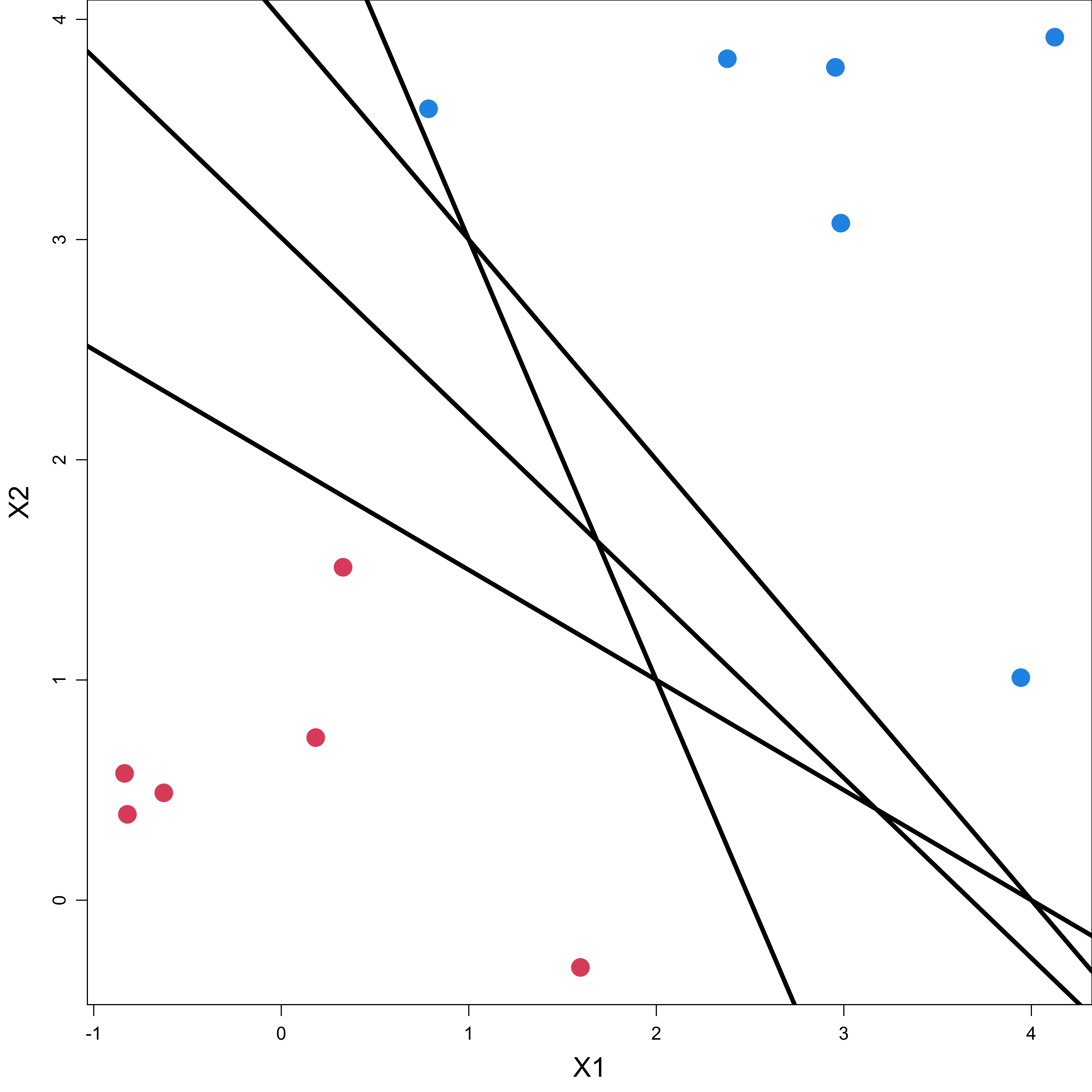
• If our data can be perfectly separated using a hyperplane, there exists an infinite number of such hyperplanes. But which one is the best?

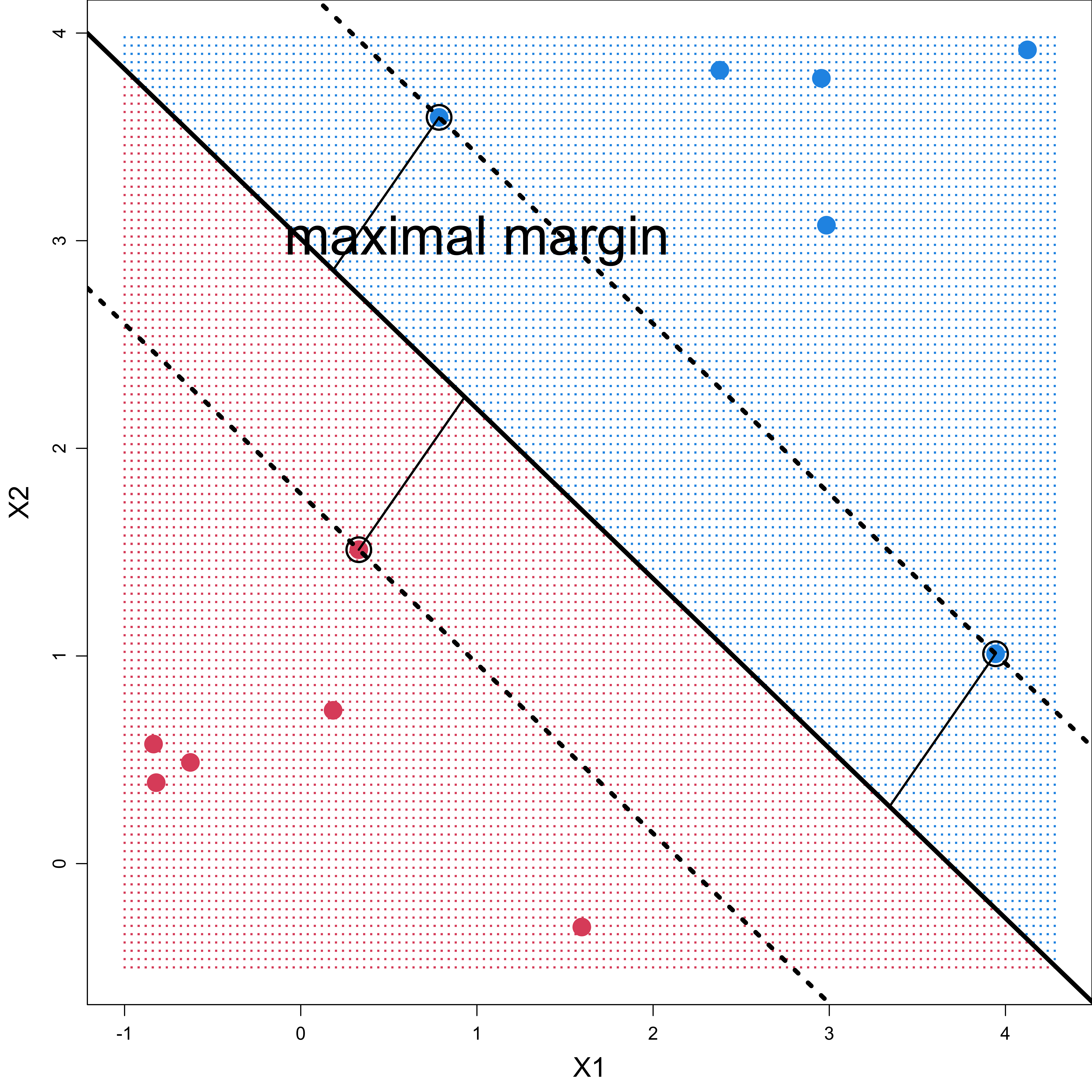
• A natural choice is the maximal margin hyperplane (optimal separating hyperplane), which is the separating hyperplane that is farthest from the training points.

Maximum-margin Classifier

library(e1071)
svm_fit <- svm(y ~ ., data = data.frame(x, y), type = 'C-classification', 
               kernel = 'linear', scale = FALSE, cost = 10000)

• The training points lied on the dashed lines are support vectors:

  • if they were moved, the maximal margin hyperplane would move too.
  • the hyperplane depends directly on the support vectors, but not on the other observations, provided that their movement does not cause it to cross the boundary.

• It can lead to overfitting when \(p\) is large.

• Hope the classifier will also have a large margin on the test data.

We use the e1071 package to fit the SVM. There is a cost parameter C , with default value 1. This parameter has a significant impact on non-separable problems. However, for our separable case, we will set this to be a very large value, meaning that the cost for having a wrong classification is very large. We also need to specify the linear kernel.

• index gives the index of all support vectors
• coefs provides the yiαi for the support vectors
• SV are the xi values correspond to the support vectors
• rho is negative β0

they “support” the maximal margin hyperplane in the sense vector that if these points were moved slightly then the maximal margin hyperplane would move as well.

https://afit-r.github.io/svm

kernlab::ksvm()

we can compute the (perpendicular) distance from each training observation to a given separating hyperplane; the smallest such distance is the minimal distance from the observations to the hyperplane, and is known as the margin. The maximal margin hyperplane is the separating hyperplane for which the margin is margin largest—that is, it is the hyperplane that has the farthest minimum distance to the training observations.

Use from sklearn import svm for Python implementation.

Linearly Separable SVM

In linear SVM, \(f(\mathbf{x}) = \beta_0 + \mathbf{x}' \boldsymbol \beta\). When \(f(\mathbf{x}) = 0\), it corresponds to a hyperplane that separates the two classes:

\[\{ \mathbf{x}: \beta_0 + \mathbf{x}'\boldsymbol \beta = 0 \}\]

• For this separable case, all observations with \(y_i = 1\) are on one side \(f(\mathbf{x}) > 0\), and observations with \(y_i = -1\) are on the other side.

• The distance from any point \(\mathbf{x}_0\) to the hyperplane is

\[\frac{1}{\lVert \boldsymbol \beta\lVert} |f(\mathbf{x}_0)|\] For \(p = 2\), and the plane \(\beta_0 + \beta_1 X_1 + \beta_2X_2 = 0\), the distance is \[ \frac{ |\beta_0 + \beta_1 x_{01} + \beta_2x_{02}|}{\sqrt{\beta_1^2 + \beta^2_2}}\]

Optimization for Linearly Separable SVM

\[\begin{align} \underset{\boldsymbol \beta, \beta_0}{\text{max}} \quad & M \\ \text{s.t.} \quad & \frac{1}{\lVert \boldsymbol \beta\lVert} y_i(\mathbf{x}' \boldsymbol \beta+ \beta_0) \geq M, \,\, i = 1, \ldots, n. \end{align}\]

• The constraint requires that each point be on the correct side of the hyperplane, with some cushion.

• The scale of \(\boldsymbol \beta\) can be arbitrary, so just set it as \(\lVert \boldsymbol \beta\rVert = 1\):

\[\begin{align} \underset{\boldsymbol \beta, \beta_0}{\text{max}} \quad & M \\ \text{s.t.} \quad & \lVert \boldsymbol \beta\lVert = 1, \\ \quad & y_i(\mathbf{x}' \boldsymbol \beta+ \beta_0) \geq M, \,\, i = 1, \ldots, n. \end{align}\]

• How to solve it? Learn it in MSSC 5650.

Linearly Non-separable SVM with Slack Variables

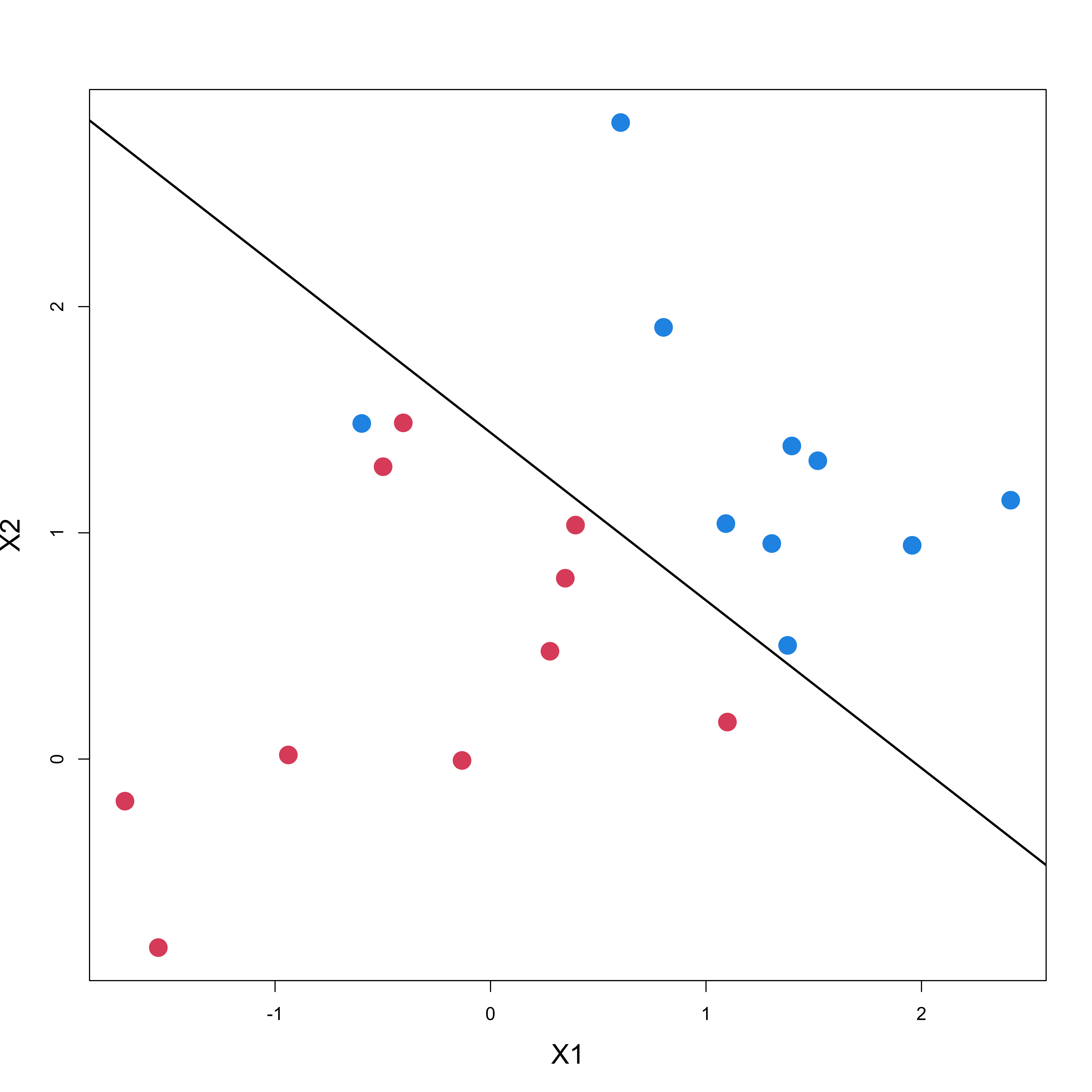
• Often, no separating hyperplane exists, so there is no maximal margin classifier.

• The previous optimization problem has no solution with \(M > 0\).

• Idea: develop a hyperplane that almost separates the classes, using a so-called soft margin: soft margin classifier.

Why Linearly Non-separable Support Vector Classifier

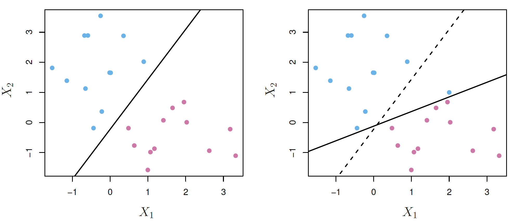
• Even if a separating hyperplane does exist, the maximum-margin classifier might not be desirable.

• The maximal margin hyperplane is extremely sensitive to a change in a single observation: it may overfit the training data. (low-bias high-variance)

Source: ISL Fig. 9.5

Soft Margin Classifier

• Consider a classifier based on a hyperplane that does NOT perfectly separate the two classes, but

  • Greater robustness to individual observations
  • Better classification of most of the training observations.

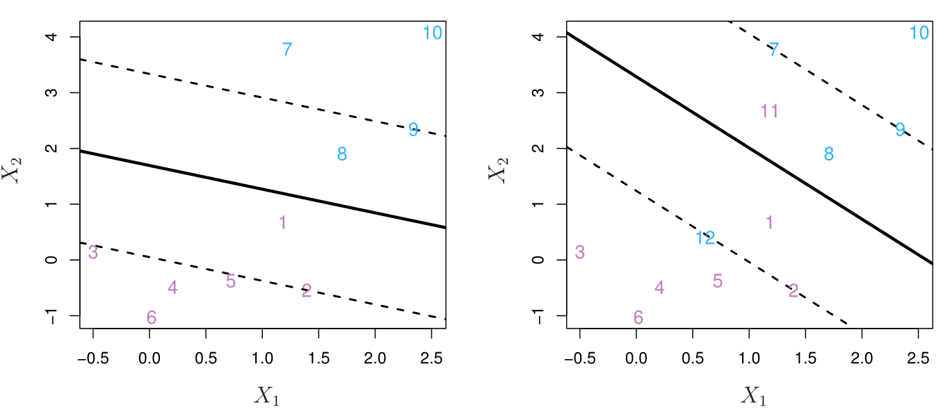
• It could be worthwhile to misclassify a few training points in order to do a better job in classifying the remaining observations.

• Allow some points to be on the incorrect side of the margin, or even the incorrect side of the hyperplane (training points misclassified by the classifier).

Source: ISL Fig. 9.6

Optimization for Soft Margin Classifier

\[\begin{align} \underset{\boldsymbol \beta, \beta_0, \epsilon_1, \dots, \epsilon_n}{\text{max}} \quad & M \\ \text{s.t.} \quad & \lVert \boldsymbol \beta\lVert = 1, \\ \quad & y_i(\mathbf{x}' \boldsymbol \beta+ \beta_0) \geq M(1 - \epsilon_i), \\ \quad & \epsilon_i \ge 0, \sum_{i=1}^n\epsilon_i \le B, \,\, i = 1, \ldots, n, \end{align}\] where \(B > 0\) is a tuning parameter.

• \(\epsilon_1, \dots, \epsilon_n\) are slack variables that allow individual points to be on slack the wrong side of the margin or the hyperplane.

• The \(i\)th point is on the

  • correct side of the margin when \(\epsilon_i = 0\)
  • wrong side of the margin when \(\epsilon_i > 0\)
  • wrong side of the hyperplane when \(\epsilon_i > 1\)

• tells us where the \(i\)th observation is located, relative to the hyperplane and relative to the margin.

Optimization for Soft Margin Classifier

\[\begin{align} \underset{\boldsymbol \beta, \beta_0, \epsilon_1, \dots, \epsilon_n}{\text{max}} \quad & M \\ \text{s.t.} \quad & \lVert \boldsymbol \beta\lVert = 1, \\ \quad & y_i(\mathbf{x}' \boldsymbol \beta+ \beta_0) \geq M(1 - \epsilon_i), \\ \quad & \epsilon_i \ge 0, \sum_{i=1}^n\epsilon_i \le B, \,\, i = 1, \ldots, n, \end{align}\] where \(B > 0\) is a tuning parameter.

• \(B\) determines the number and severity of the violations to the margin/hyperplane we tolerate.
  • \(B = 0\): no budget for violations (\(\epsilon_1 = \cdots = \epsilon_n = 0\))
  • \(B > 0\): no more than \(B\) points can be on the wrong side of the hyperplane. (\(\epsilon_i > 1\))
  • As \(B\) increases, more violations and wider margin. (more bias less variance)
  • Choose \(B\) via cross-validation.

B as a budget for the amount that the margin can be violated by the n observations

Optimization for Soft Margin Classifier

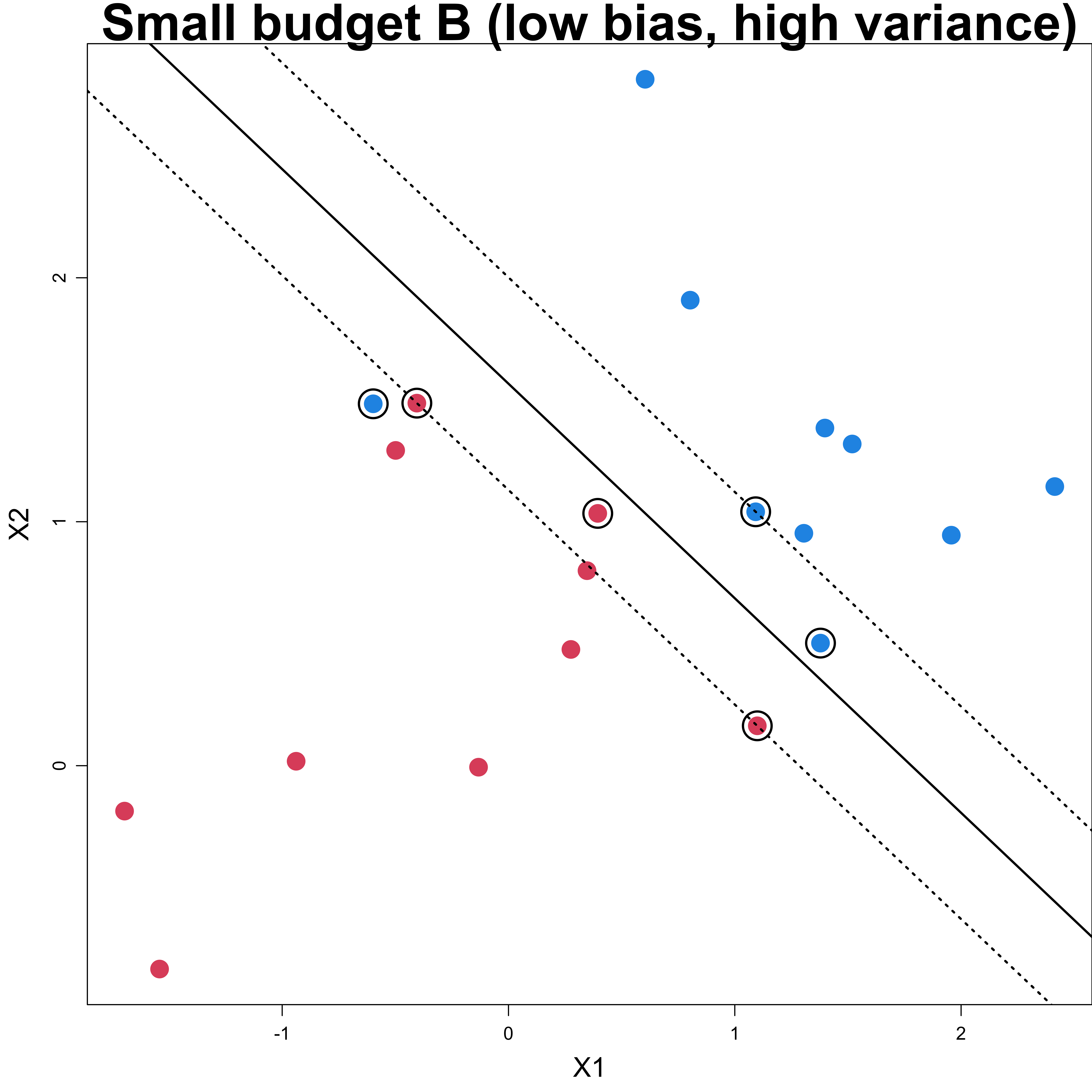
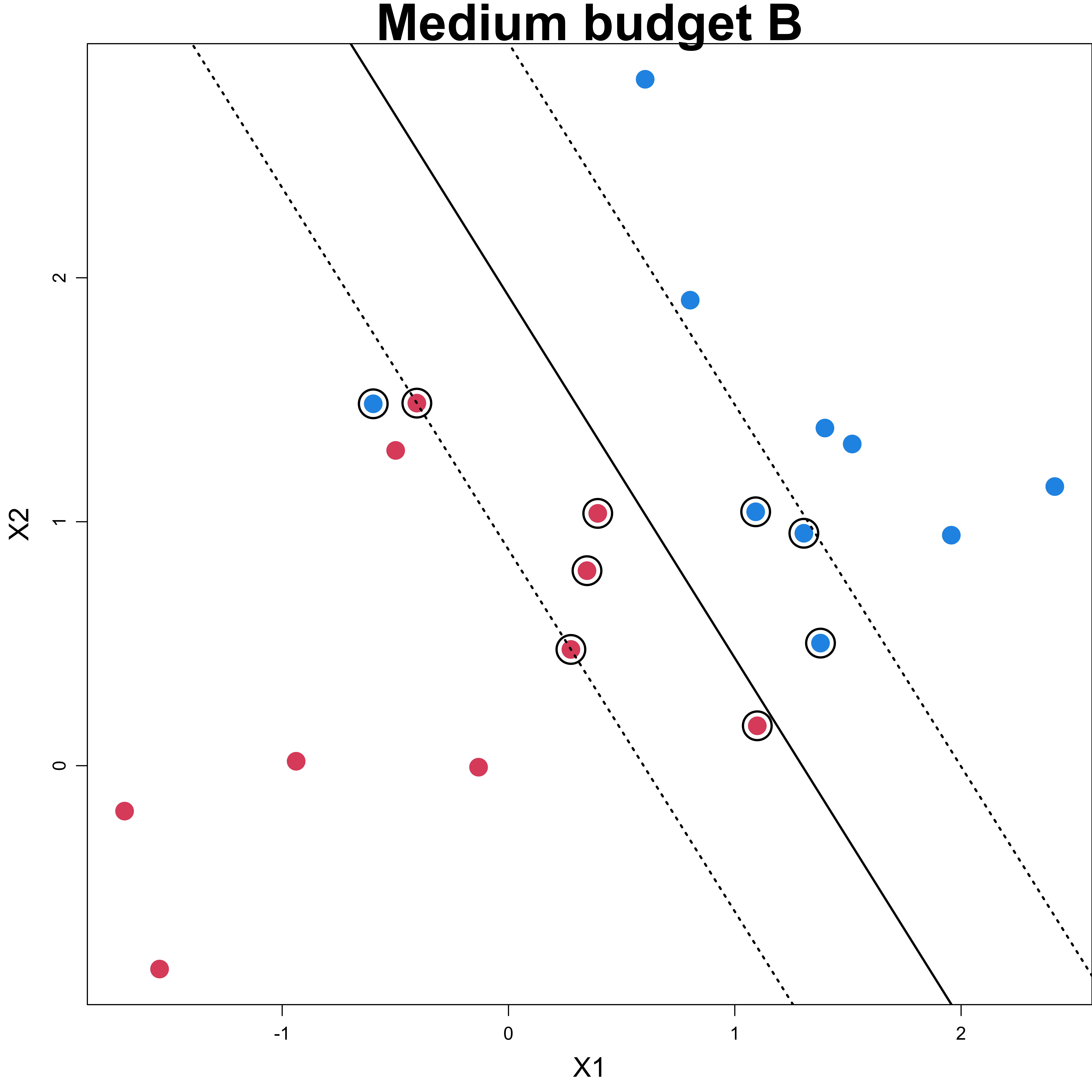
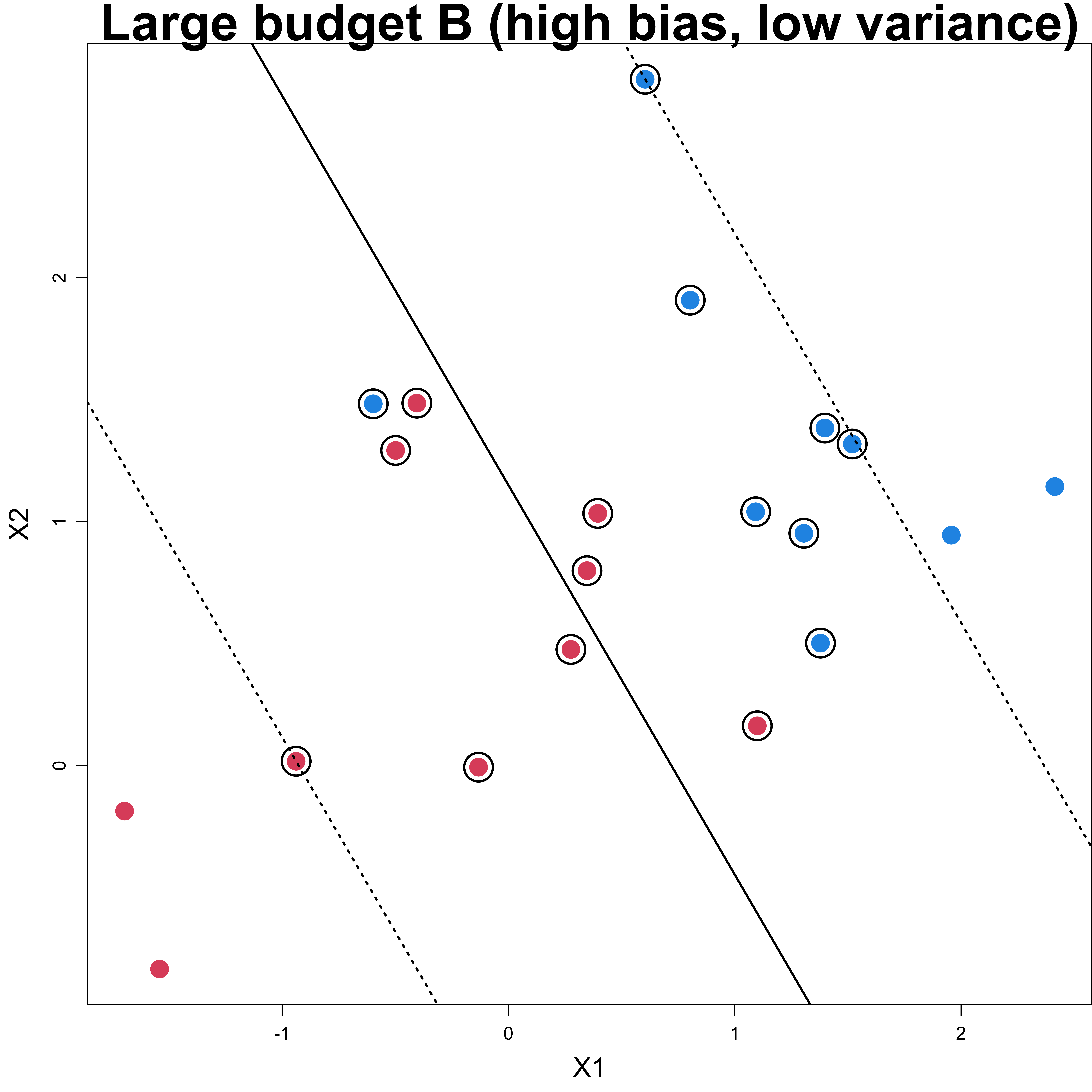
Optimization for Soft Margin Classifier

Warning

The argument cost in e1071::svm() is the \(C\) defined in the primal form \[\begin{align} \underset{\boldsymbol \beta, \beta_0}{\text{min}} \quad & \frac{1}{2}\lVert \boldsymbol \beta\rVert^2 + C \sum_{i=1}^n \epsilon_i \\ \text{s.t} \quad & y_i (\mathbf{x}_i' \boldsymbol \beta+ \beta_0) \geq (1 - \epsilon_i), \\ \text{} \quad & \epsilon_i \geq 0, \,\, i = 1, \ldots, n, \end{align}\]

so small cost \(C\) means larger budget \(B\).

SVM, LDA and Logistic Regression

Note

• SVM decision rule is based only on a subset of the training data (robust to the behavior of data that are far away from the hyperplane.)

• LDA depends on the mean of all of the observations within each class, and within-class covariance matrix computed using all of the data.

• Logistic regression, unlike LDA, is insensitive to observations far from the decision boundary too.

Classification with Non-Linear Decision Boundaries

• The soft margin classifier is a natural approach for classification in the two-class setting, if the boundary between the two classes is linear.

• In practice we are often faced with non-linear class boundaries.

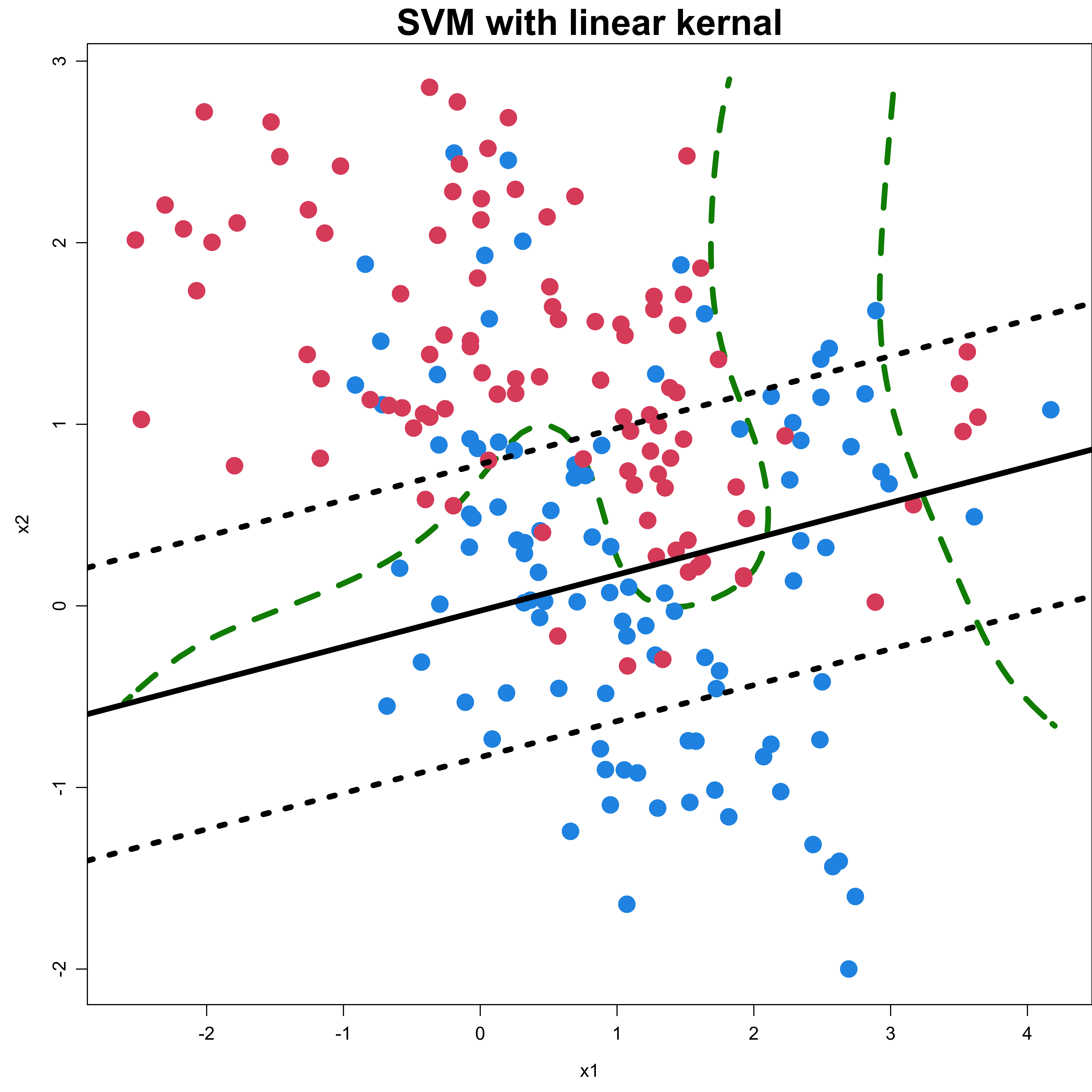
Classification with Non-Linear Decision Boundaries

• In regression, we enlarge the feature space using functions of the predictors to address this non-linearity.

• In SVM (logistic regression too!), we could address non-linear boundaries by enlarging the feature space.

• For example, rather than fitting a support vector classifier using \(p\) features, \(X_1, \dots, X_p\), we could instead fit a support vector classifier using \(2p\) features \(X_1,X_1^2,X_2,X_2^2, \dots , X_p, X_p^2\).

\[\begin{align} \underset{\beta_0, \beta_{11}, \beta_{12}, \dots, \beta_{p1}, \beta_{p2}, \epsilon_1, \dots, \epsilon_n}{\text{max}} \quad & M \\ \text{s.t.} \quad & y_i\left(\beta_0 + \sum_{i = 1}^n \beta_{j1}x_{ij} + \sum_{i = 1}^n \beta_{j2}x_{ij}^2\right) \geq M(1 - \epsilon_i), \\ \quad & \epsilon_i \ge 0, \sum_{i=1}^n\epsilon_i \le B, \,\, i = 1, \ldots, n,\\ \quad & \sum_{j=1}^p\sum_{k=1}^2\beta_{jk}^2 = 1. \end{align}\]

In the enlarged feature space, the decision boundary that results from (9.16) is in fact linear. But in the original feature space, the decision boundary is of the form q(x) = 0, where q is a quadratic polynomial, and its solutions are generally non-linear.

The support vector machine, which we present next, allows us to enlarge the feature space used by the support vector classifier in a way that leads to efficient computations

Solution to Support Vector Classifier

• The solution to the support vector classifier optimization involves only the inner products of the observations: \(\langle \mathbf{x}_i, \mathbf{x}_{i'} \rangle = \sum_{j=1}^px_{ij}x_{i'j}\)

• The linear support vector classifier can be represented as \[f(\mathbf{x}) = \beta_0 + \sum_{i\in \mathcal{S}}\alpha_i\langle \mathbf{x}, \mathbf{x}_{i} \rangle\] where \(\mathcal{S}\) is the collection of indices of the support points.

• \(\alpha_i\) is nonzero only for the support vectors in the solution

• To evaluate the function \(f(\mathbf{x}_0)\), we compute \(\langle \mathbf{x}_0, \mathbf{x}_{i} \rangle\).

Nonlinear SVM via Kernel Trick

• The support vector machine (SVM) is an extension of the support vector classifier that results from enlarging the feature space in a specific way, using kernels.

• The kernel approach is an efficient computational approach for enlarging our feature space and non-linear boundary.

• Kernel Trick: \[f(\mathbf{x}) = \beta_0 + \sum_{i\in \mathcal{S}}\alpha_i K\left(\mathbf{x}, \mathbf{x}_{i}\right) \]

• Linear kernel: \(K\left(\mathbf{x}_0, \mathbf{x}_{i}\right) = \langle \mathbf{x}_0, \mathbf{x}_{i'} \rangle = \sum_{j=1}^px_{0j}x_{ij}\)

• Polynomial kernel: \(K\left(\mathbf{x}_0, \mathbf{x}_{i}\right) = \left(1 + \sum_{j=1}^px_{0j}x_{ij}\right)^d\)

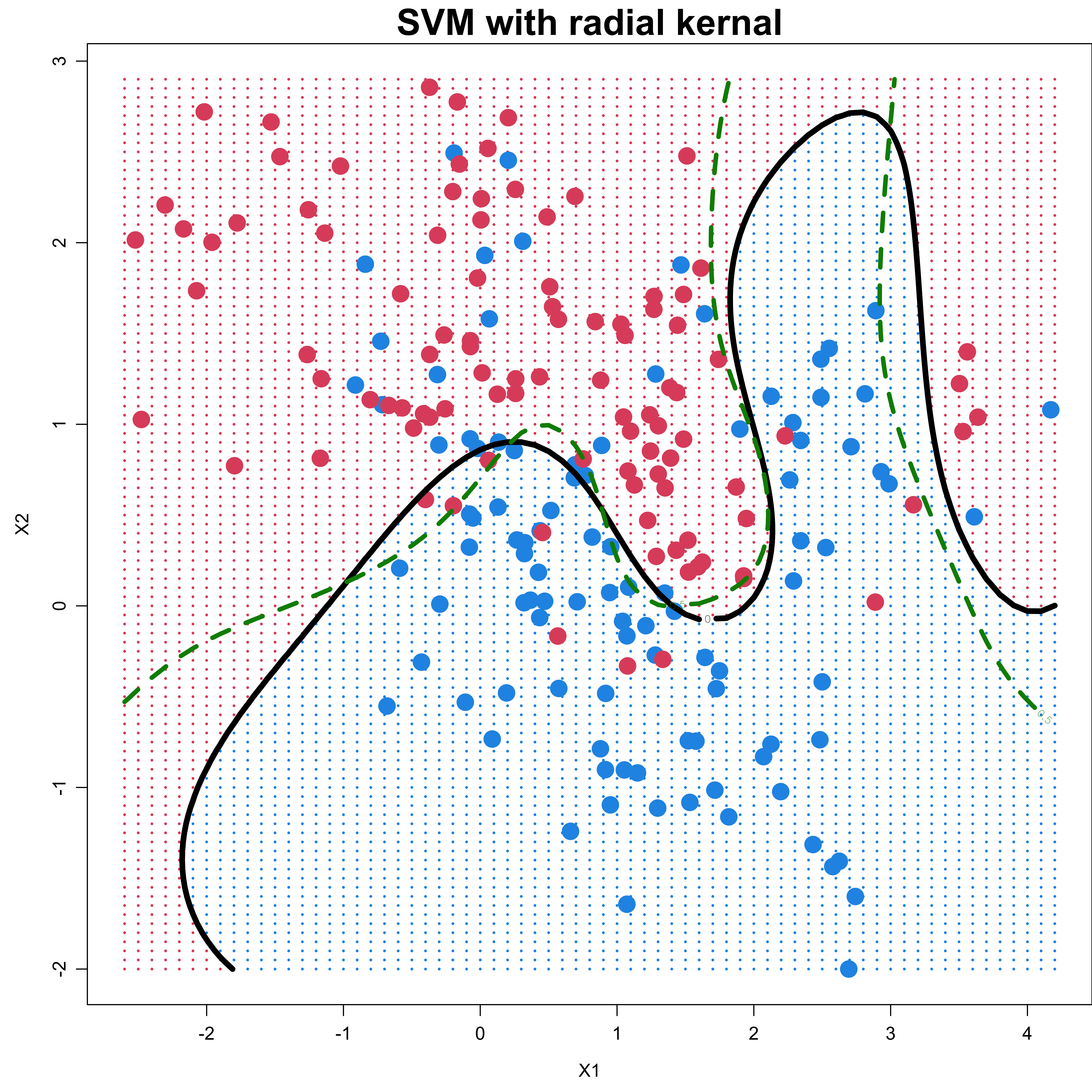
• Radial kernel: \(K\left(\mathbf{x}_0, \mathbf{x}_{i'}\right) = \exp \left(-\gamma\sum_{j=1}^p (x_{0j}-x_{ij})^2 \right)\)

Radial Kernel Decision Doundary

SVM as a Penalized Model

\[\begin{align} \underset{\boldsymbol \beta, \beta_0, \epsilon_1, \dots, \epsilon_n}{\text{max}} \quad & M \\ \text{s.t.} \quad & \lVert \boldsymbol \beta\lVert = 1, \\ \quad & y_i(\mathbf{x}_i' \boldsymbol \beta+ \beta_0) \geq M(1 - \epsilon_i), \\ \quad & \epsilon_i \ge 0, \sum_{i=1}^n\epsilon_i \le B, \,\, i = 1, \ldots, n, \end{align}\]

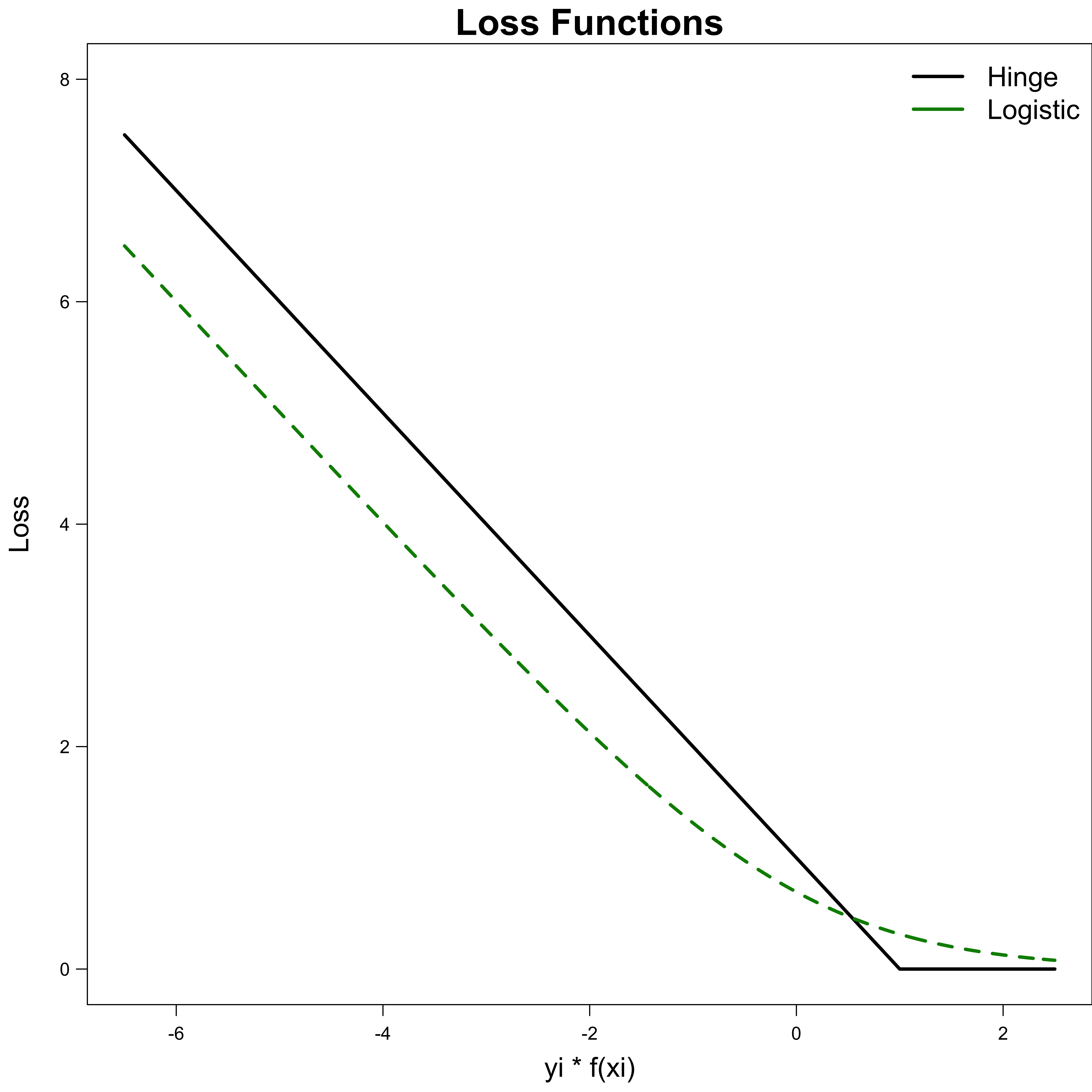
\[\begin{align} \underset{\boldsymbol \beta, \beta_0}{\text{min}} \left\{ \sum_{i=1}^n \max \left[ 0, 1 - y_i (\mathbf{x}_i' \boldsymbol \beta+ \beta_0) \right] + \lambda \lVert \boldsymbol \beta\lVert ^ 2 \right\} \end{align}\] where \(\sum_{i=1}^n \max \left[ 0, 1 - y_i (\mathbf{x}' \boldsymbol \beta+ \beta_0) \right]\) is known as hinge loss.

• Large \(\lambda\) (large \(B\)): small \(\beta_j\)s, high-bias and low-variance.

• Small \(\lambda\) (small \(B\)): low-bias and high-variance.

Loss Functions

• The hinge loss is zero for observations for which \(y_i (\mathbf{x}' \boldsymbol \beta+ \beta_0) \ge 1\) (correct side of the margin).

• The logistic loss is not zero anywhere.

• SVM is better when classes are well separated.

• Logistic regression is preferred in more overlapping regimes.

, but small for points far from the boundary.