Clustering
MSSC 6250 Statistical Machine Learning
Department of Mathematical and Statistical Sciences
Marquette University
Clustering Methods
- Clustering: techniques for finding subgroups, or clusters, in a data set.
- Goal: Homogeneous within groups; heterogeneous between groups
-
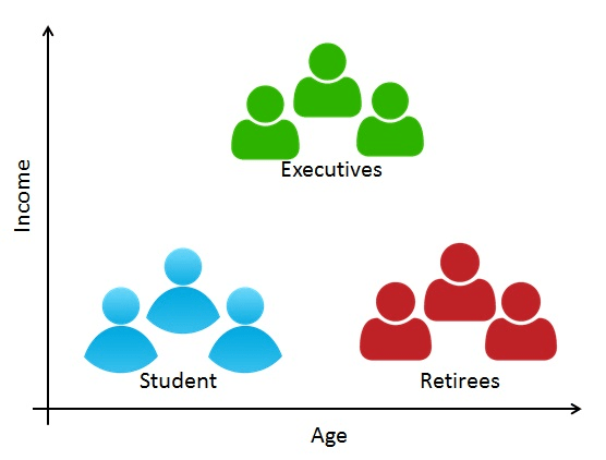
Customer/Marketing Segmentation
- Divide customers into clusters on age, income, etc.
- Each subgroup might be more receptive to a particular form of advertising, or more likely to purchase a particular product.
Source: https://shopup.me/blog/customer-segmentation-definition/
Clustering Methods
Basic clustering approaches include K-means clustering and hierarchical clustering.
Clustering results are dependent on the measure of similarity (or distance) between the data points.
For continuous variables, the most commonly used measure is the Euclidian distance: \[d(u, v) = \|u - v\|_2 = \sqrt{\sum_{j=1}^p(u_j - v_j)^2}\]
For categorical variables, the Hamming distance is usually used: \[d(u, v) = \sum_{j=1}^p \mathbf{1}\{u_j \ne v_j\}\]
Distance measures should be defined based on the application. There is no universally best approach.
K-Means Clustering
K-Means Clustering
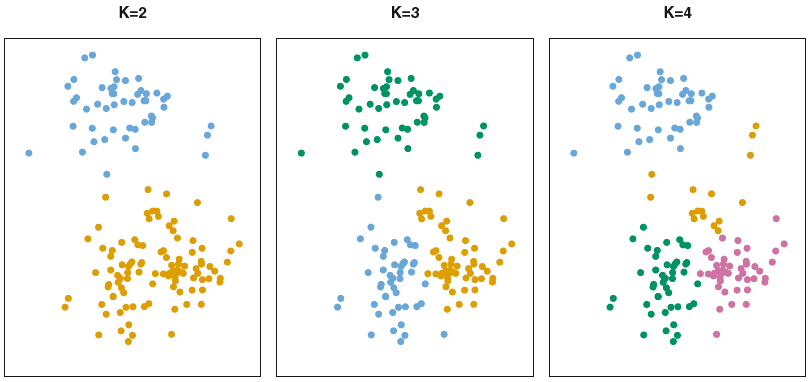
Partition observations into \(K\) distinct, non-overlapping clusters: assign each to exactly one of the \(K\) clusters.
Must pre-specify the number of clusters \(K \ll n\).
Source: Fig. 12.7 of ISL
K-Means Illustration
Data (Let’s choose \(K=2\))
K-Means Algorithm
- Choose a value of \(K\).
- Randomly assign a number, from 1 to \(K\), to each of the observations.
- Iterate until the cluster assignments stop changing:
- [1] For each of the \(K\) clusters, compute its cluster centroid.
- [2] Assign each observation to the cluster whose centroid is closest.
K-Means Illustration
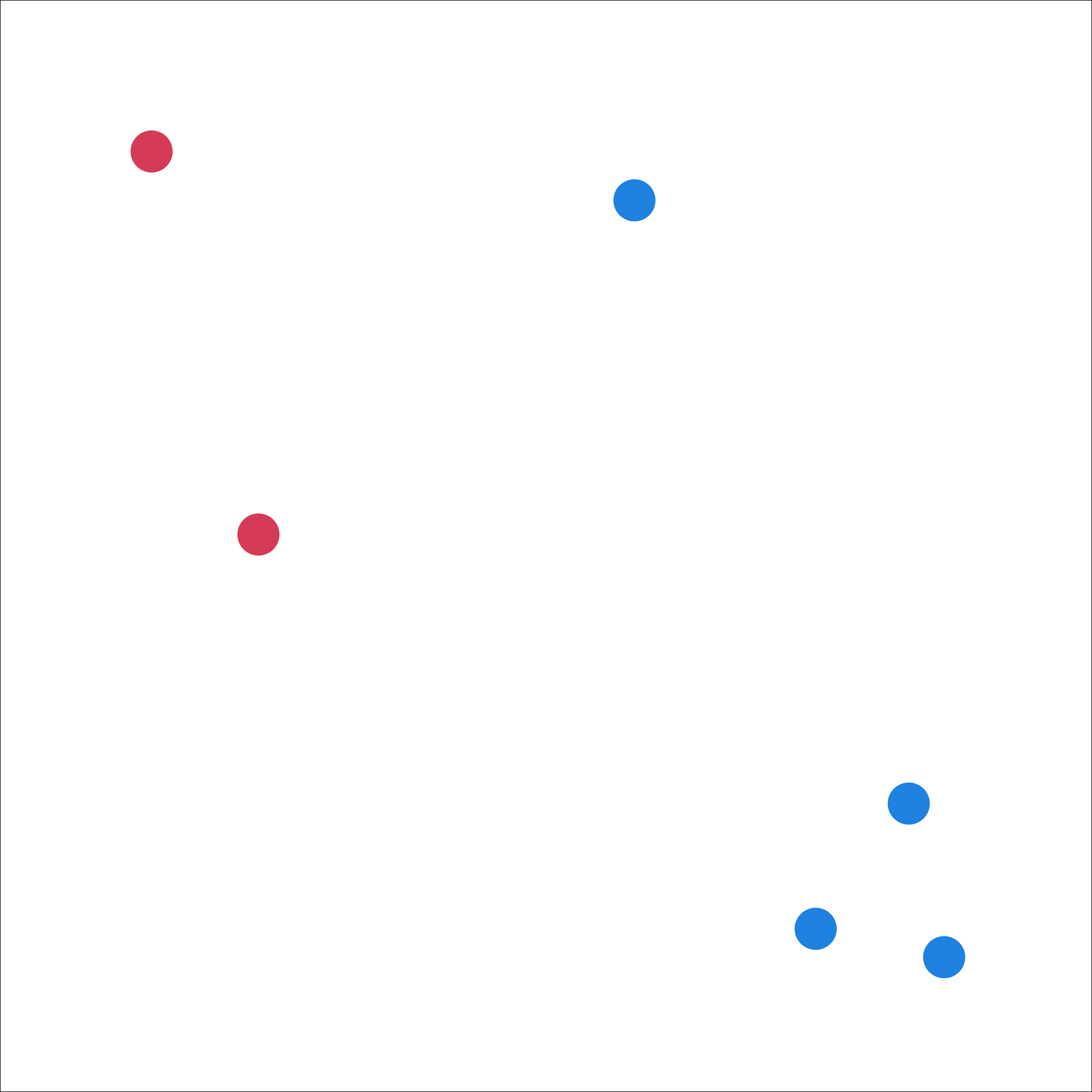
Random assignment
K-Means Algorithm
- Choose a value of \(K\).
- Randomly assign a number, from 1 to \(K\), to each of the observations.
- Iterate until the cluster assignments stop changing:
- [1] For each of the \(K\) clusters, compute its cluster centroid.
- [2] Assign each observation to the cluster whose centroid is closest.
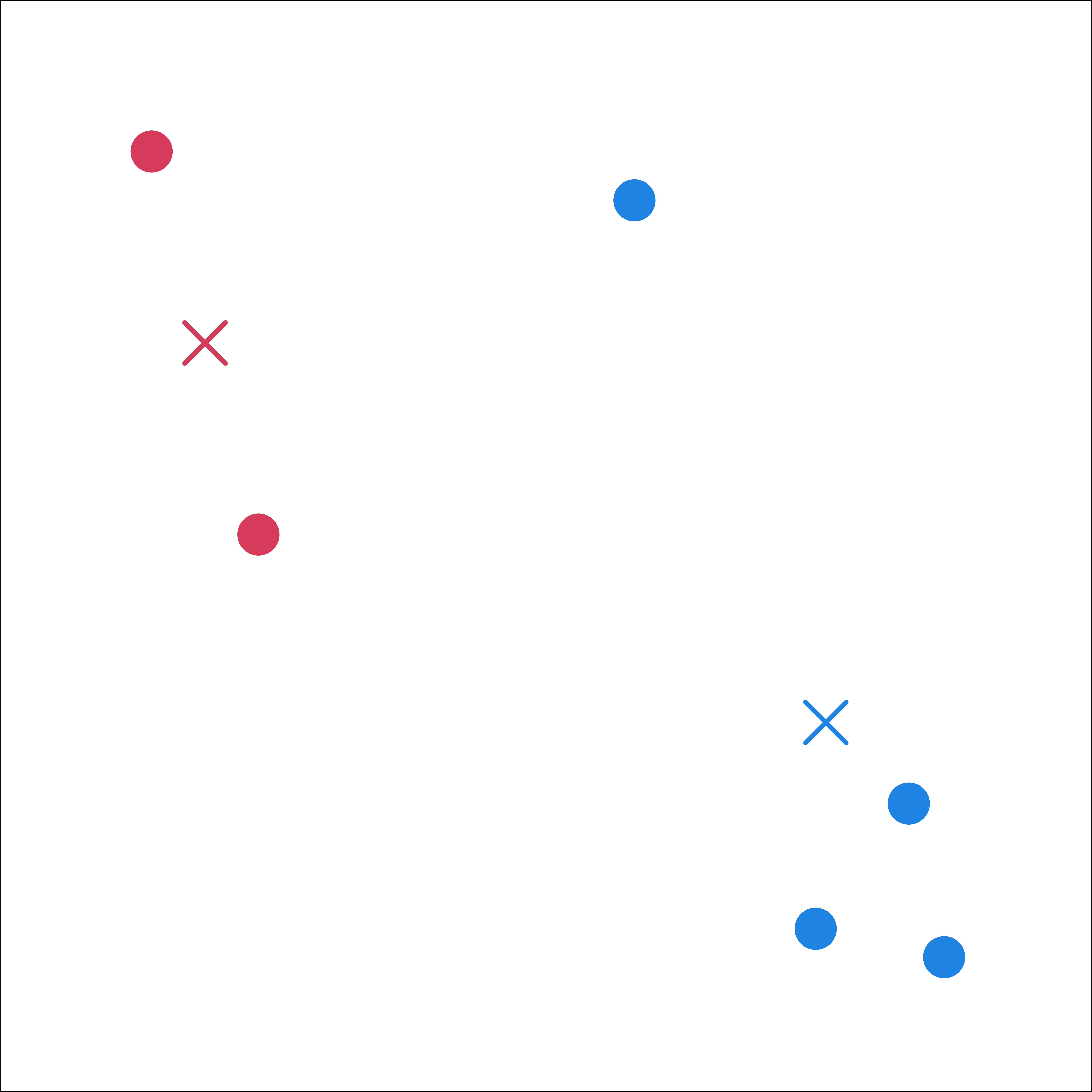
K-Means Illustration
Compute the cluster centroid
K-Means Algorithm
- Choose a value of \(K\).
- Randomly assign a number, from 1 to \(K\), to each of the observations.
- Iterate until the cluster assignments stop changing:
- [1] For each of the \(K\) clusters, compute its cluster centroid.
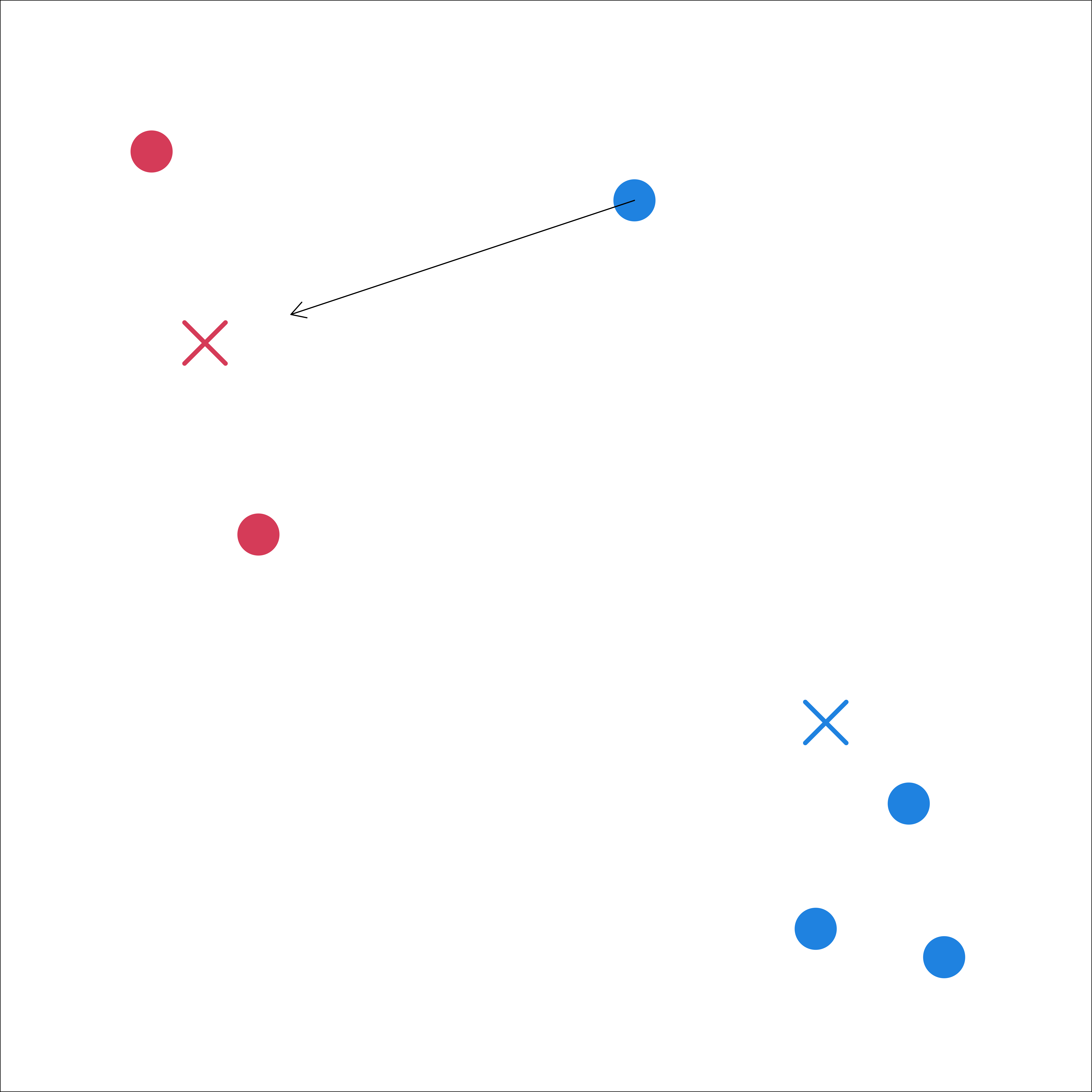
- [2] Assign each observation to the cluster whose centroid is closest.
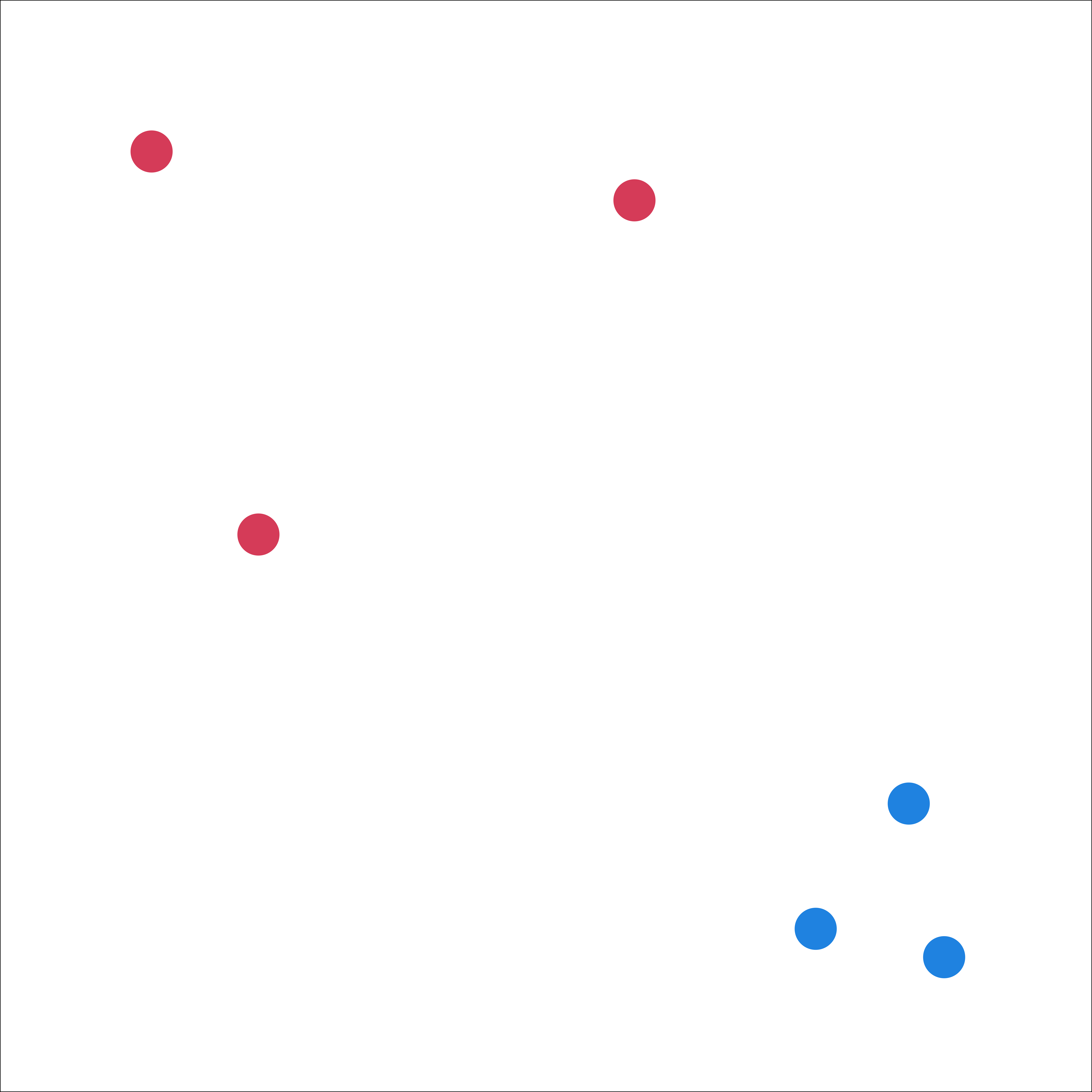
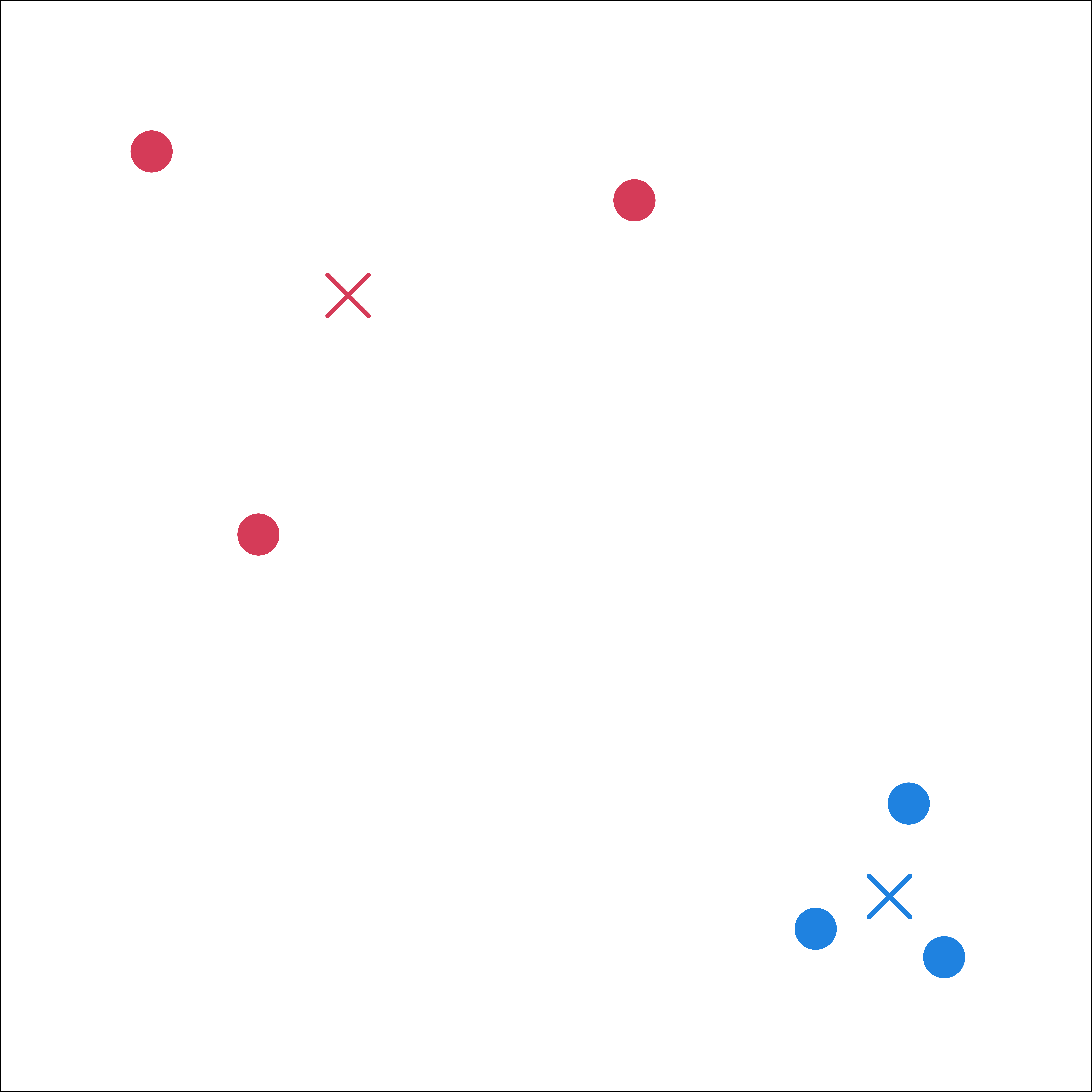
K-Means Illustration
Do a new assignment
Compute the cluster centroid
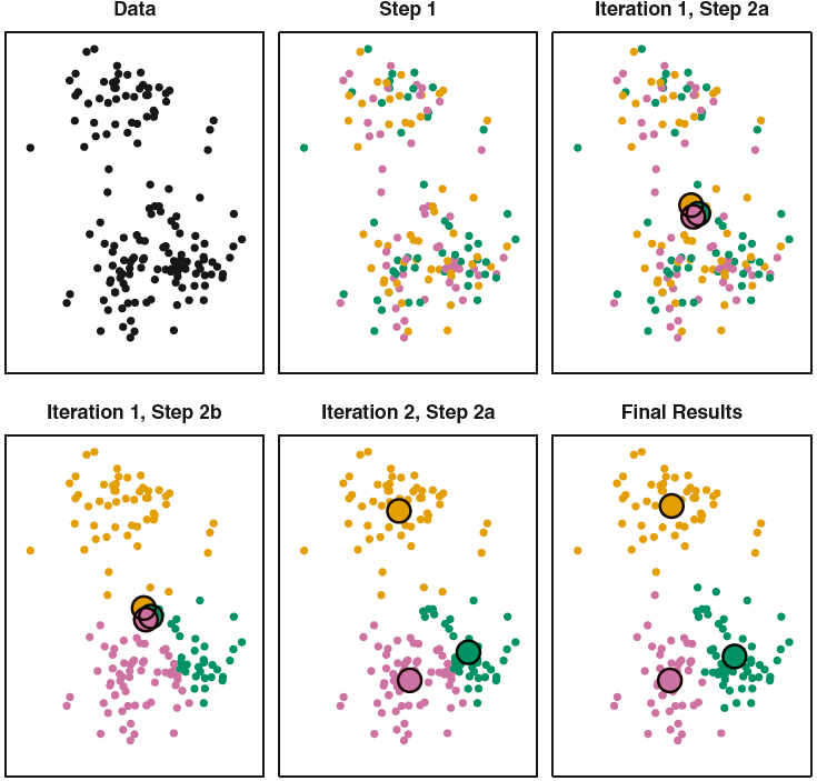
Source: ISL Figure 12.8
Clustering Mathematical Formulation
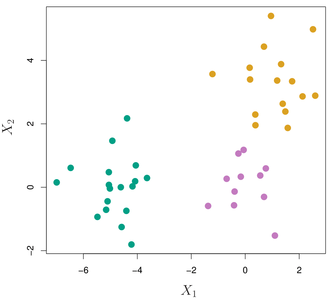
- \(C(\cdot): \{1, \ldots, n\} \rightarrow \{1, \ldots, K\}\) is a cluster assignment function or encoder that assigns the \(i\)th observation to the \(k\)th cluster, \(i \in \{1, \ldots, n\}\), \(k \in \{1, \ldots, K\}\), or \(C(i) = k\).
Seek a \(C(\cdot)\) that minimizes the within-cluster distance \[ \begin{align} W(C) = \frac{1}{2}\sum_{k=1}^K\sum_{(i, i'): C(i), C(i')=k} d(\mathbf{x}_i, \mathbf{x}_{i'}) \end{align} \]
If \(d(\cdot, \cdot)\) is the Euclidean distance, \[W(C) =\sum_{k=1}^K n_k \sum_{C(i) = k} \lVert \mathbf{x}_i - m_k \rVert^2,\]
where \(m_k = (\bar{x}_{1k}, \dots, \bar{x}_{pk})\) is the mean vector of \(k\)th cluster.
Clustering Mathematical Formulation
- This is equivalent to maximizing the between cluster distance
\[B(C) = \frac{1}{2}\sum_{k=1}^K\sum_{(i, i'): C(i)=k}\sum_{, C(i')\ne k} d(\mathbf{x}_i, \mathbf{x}_{i'})\]
- The total distance is
\[T = \frac{1}{2}\sum_{i=1}^n \sum_{i'=1}^nd(\mathbf{x}_i, \mathbf{x}_{i'}) = W(C) + B(C)\]
\[\min_{C} W(C) \iff \max_{C} B(C)\]

K-Means Clustering
- K-Means clustering use an iterative algorithm to solve the enlarged optimization problem:
\[ \underset{C, \, \{m_k\}_{k=1}^K} \min \sum_{k=1}^K n_k \sum_{C(i) = k} \lVert \mathbf{x}_i - m_k \rVert^2, \]
where \(m_k = (\bar{x}_{1k}, \dots, \bar{x}_{pk})\) is the mean vector of \(k\)th cluster.1
K-Means Algorithm Issues
The algorithm finds a local rather than a global optimum.
-
The results will depend on the initial (random) cluster assignment.
- Run the algorithm multiple times, then select the one producing the smallest \(W(C)\)
Standardize the data so that distance is not affected by variable unit.
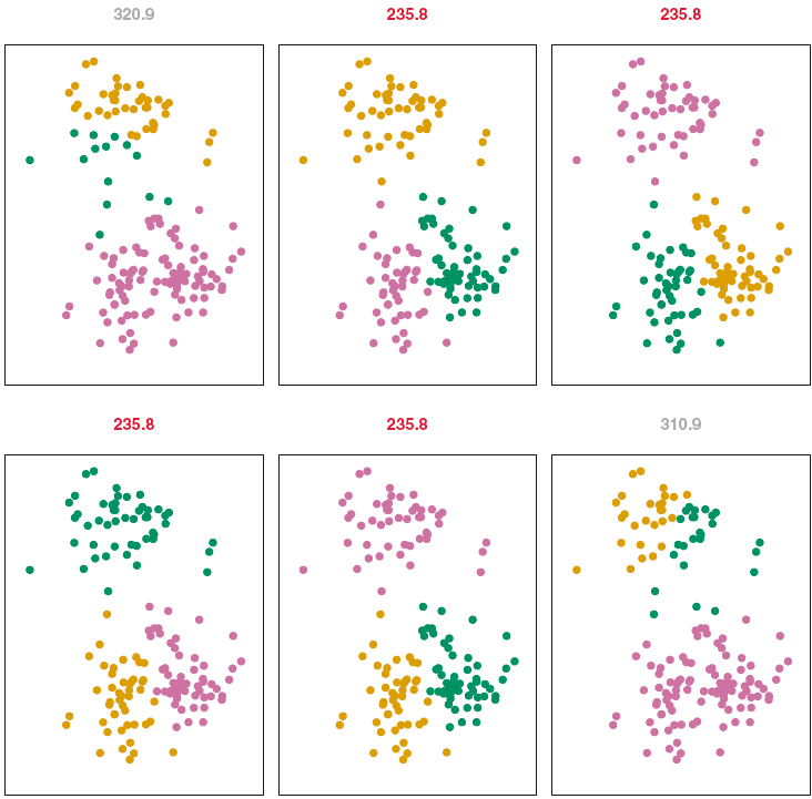
Source: ISL Figure 12.8
K-Mediods
K-medoids is an alternative of K-means.
Seek one observation that minimizes the distance to all others in the cluster \[i^*_k = \mathop{\mathrm{arg\,min}}_{i:C(i)=k}\sum_{C(i')=k}d(\mathbf{x}_i, \mathbf{x}_{i'})\]
Use \(\mathbf{x}_{i^*_k}\) as the “center” of cluster \(k\).
iris Data
  Sepal.Length Sepal.Width Petal.Length Petal.Width Species
1          5.1         3.5          1.4         0.2  setosa
2          4.9         3.0          1.4         0.2  setosa
3          4.7         3.2          1.3         0.2  setosa
4          4.6         3.1          1.5         0.2  setosa
5          5.0         3.6          1.4         0.2  setosa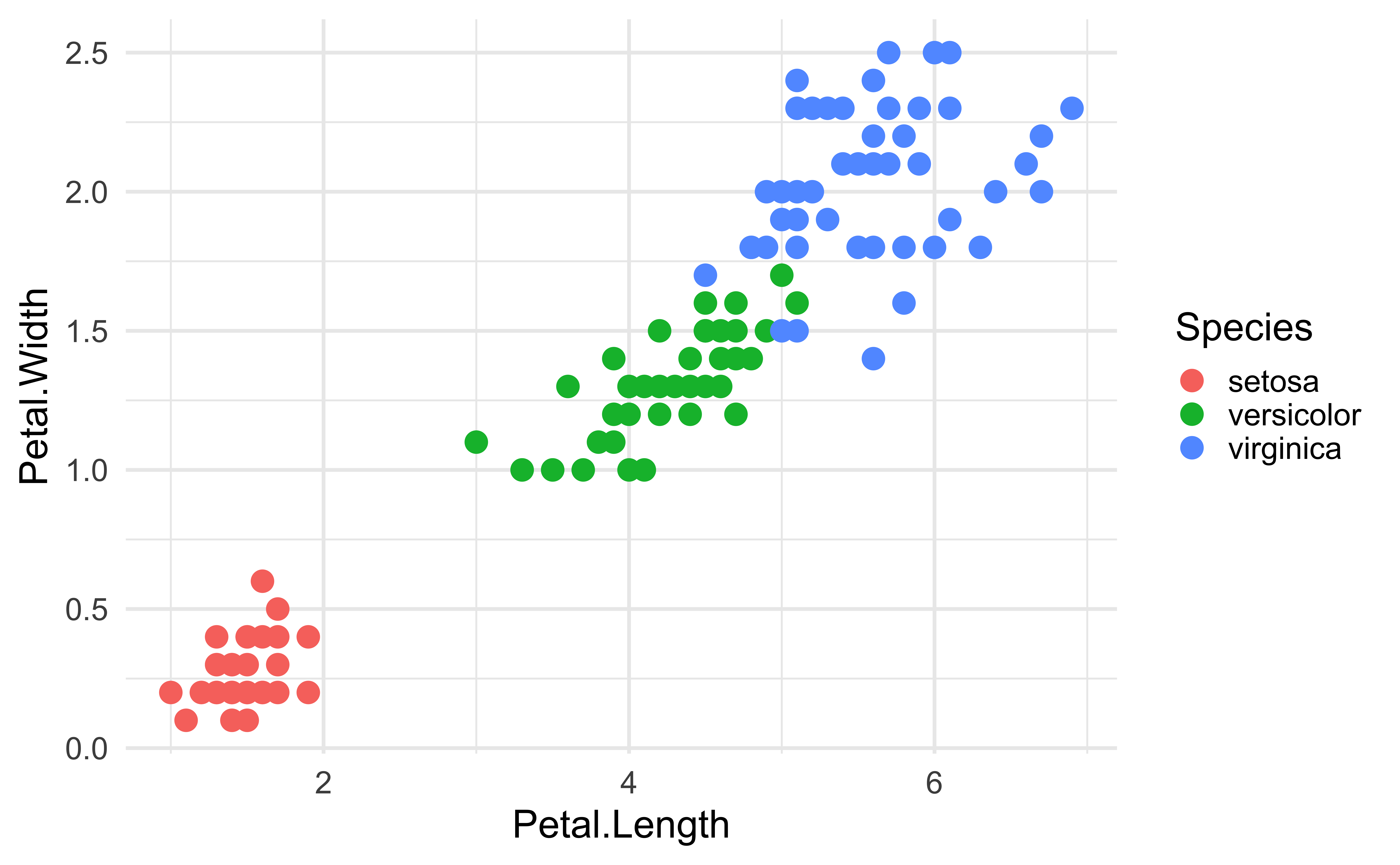
K-Means on iris
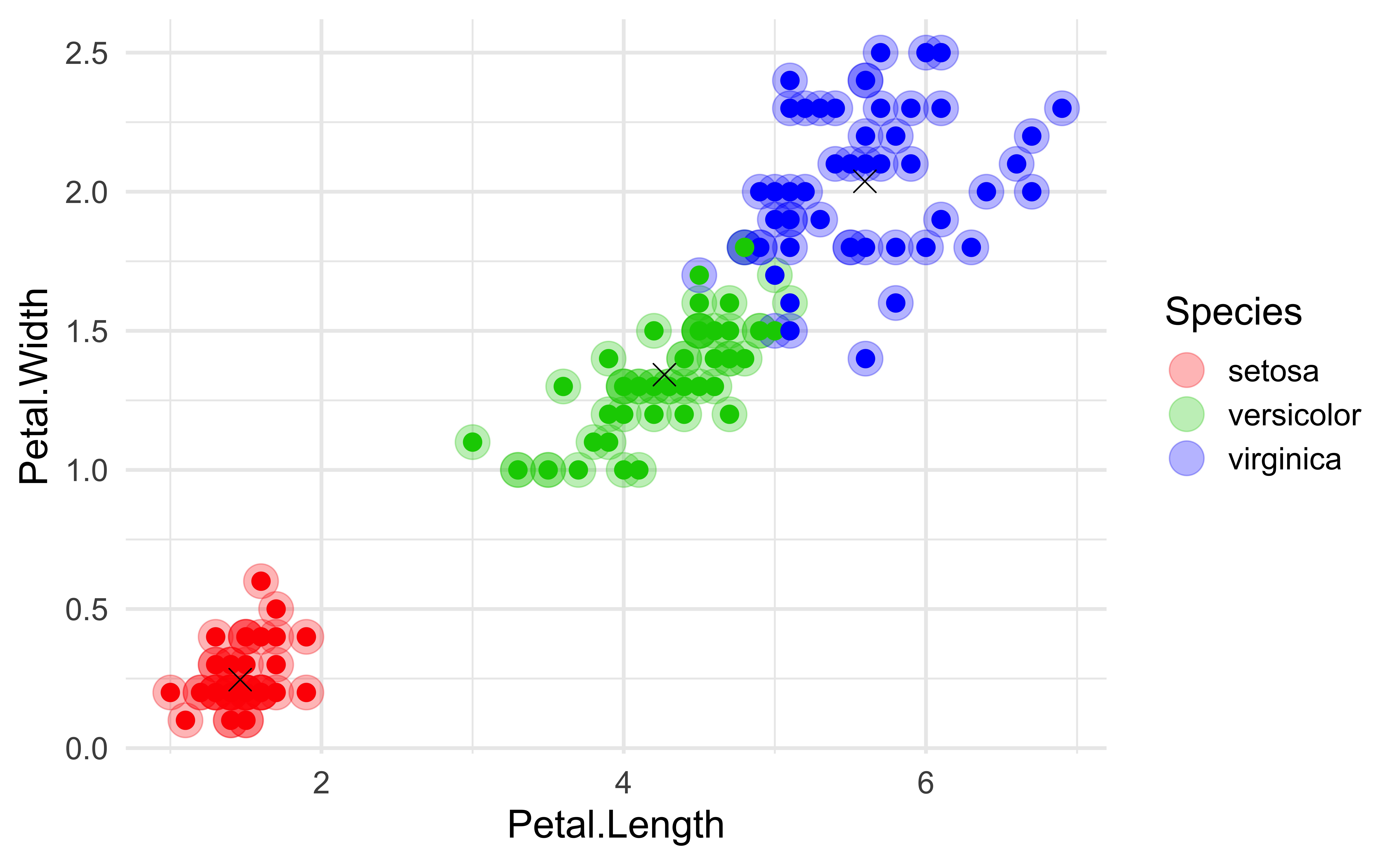
K-means clustering with 3 clusters of sizes 50, 48, 52

Cluster means:
  Petal.Length Petal.Width
1         1.46       0.246
2         5.60       2.037
3         4.27       1.342

Clustering vector:
  [1] 1 1 1 1 1 1 1 1 1 1 1 1 1 1 1 1 1 1 1 1 1 1 1 1 1 1 1 1 1 1 1 1 1 1 1 1 1
 [38] 1 1 1 1 1 1 1 1 1 1 1 1 1 3 3 3 3 3 3 3 3 3 3 3 3 3 3 3 3 3 3 3 3 3 3 3 3
 [75] 3 3 3 2 3 3 3 3 3 2 3 3 3 3 3 3 3 3 3 3 3 3 3 3 3 3 2 2 2 2 2 2 3 2 2 2 2
[112] 2 2 2 2 2 2 2 2 3 2 2 2 2 2 2 3 2 2 2 2 2 2 2 2 2 2 2 3 2 2 2 2 2 2 2 2 2
[149] 2 2

Within cluster sum of squares by cluster:
[1]  2.02 16.29 13.06
 (between_SS / total_SS =  94.3 %)

Available components:

[1] "cluster"      "centers"      "totss"        "withinss"     "tot.withinss"
[6] "betweenss"    "size"         "iter"         "ifault"
K-Means on iris
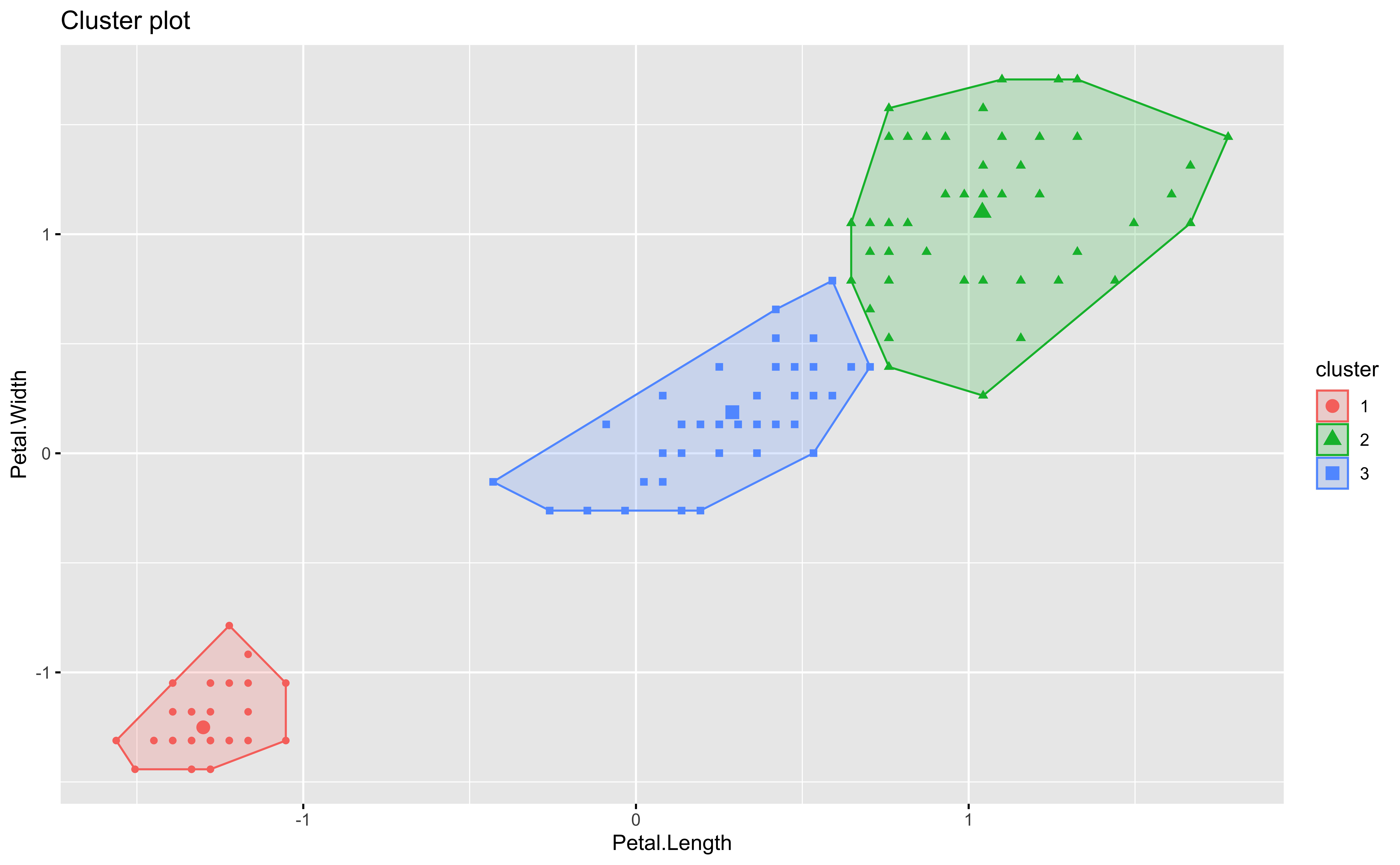
factoextra
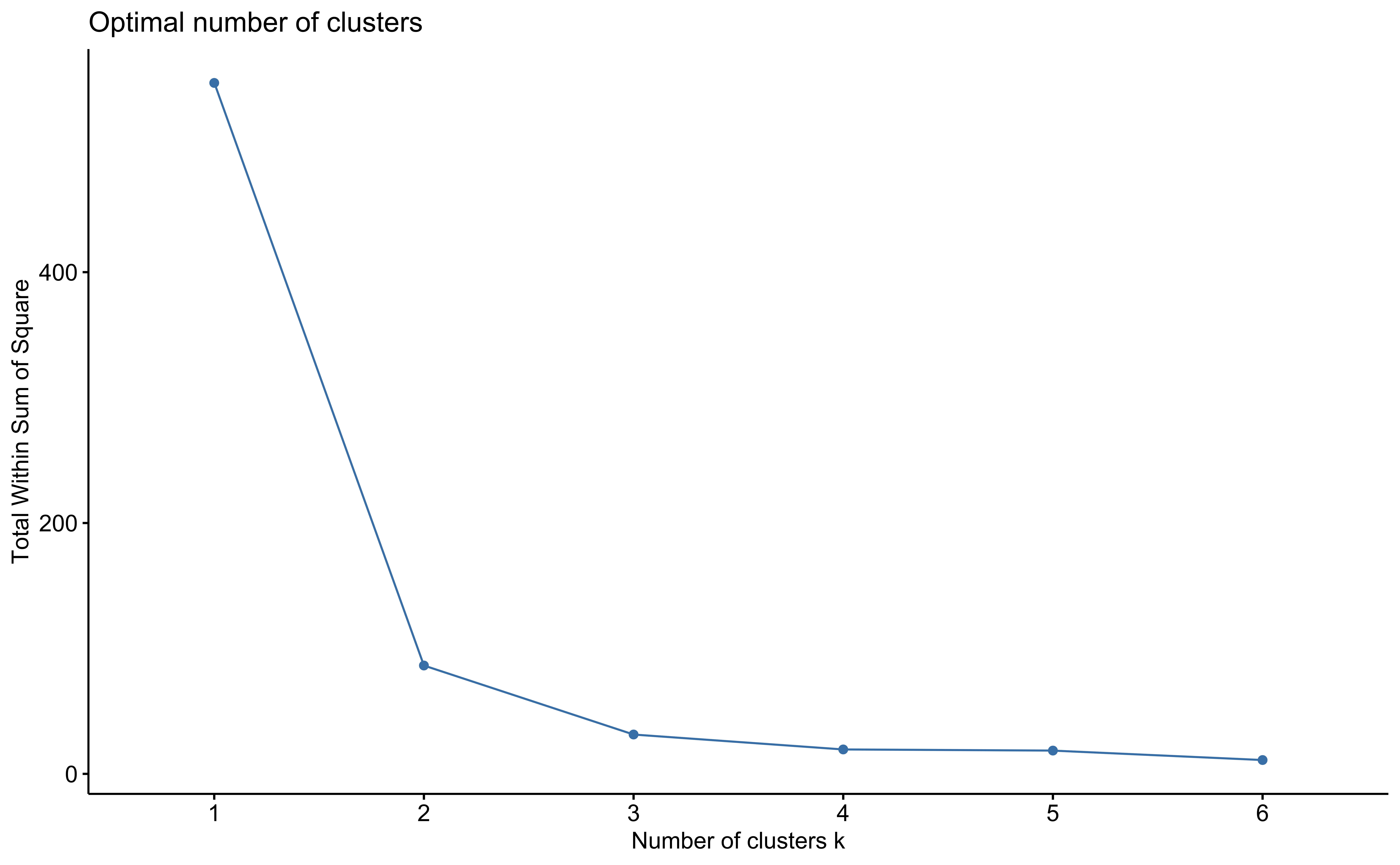
Choose K: Total Withing Sum of Squares
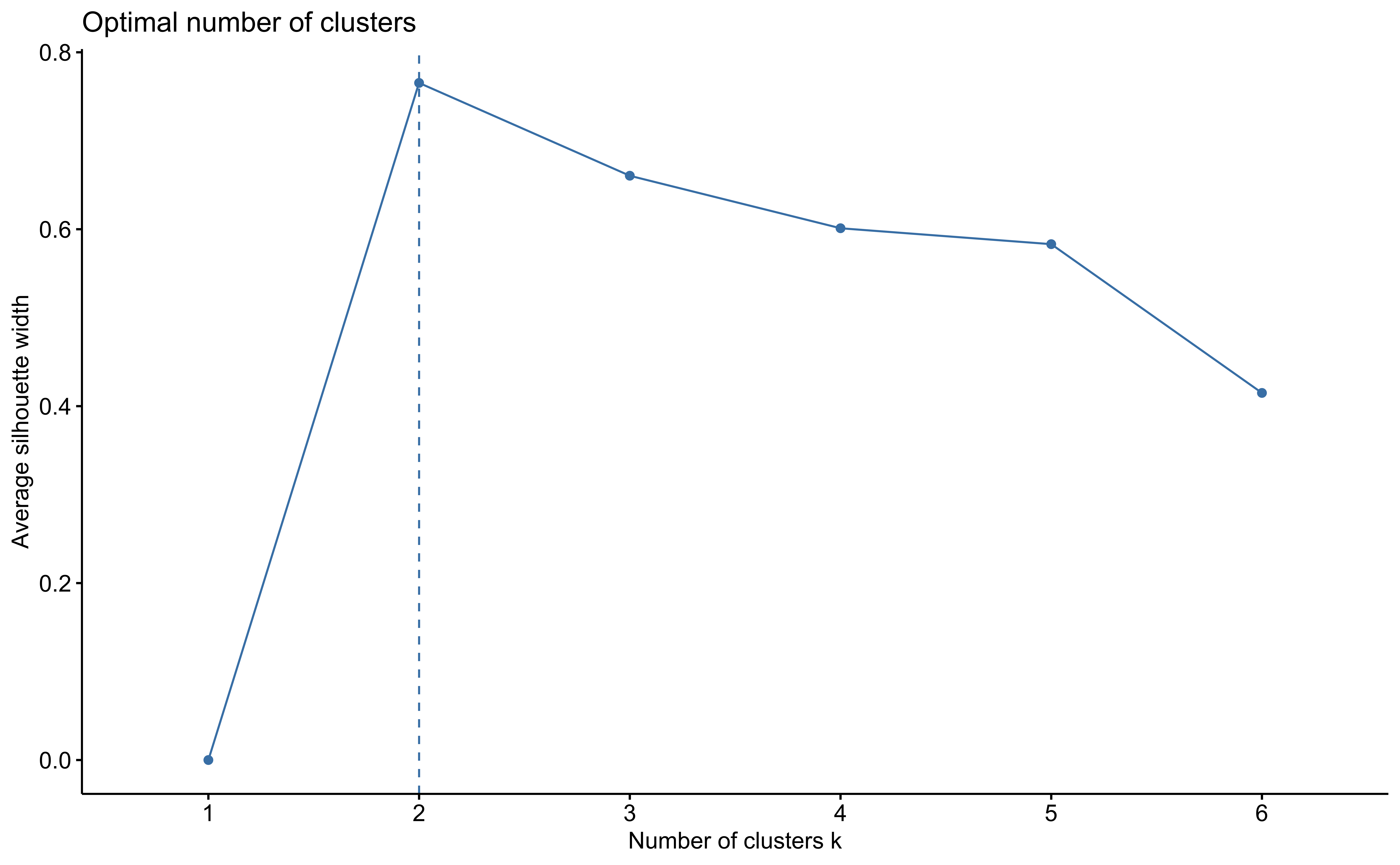
Choose K: Average Silhouette Method
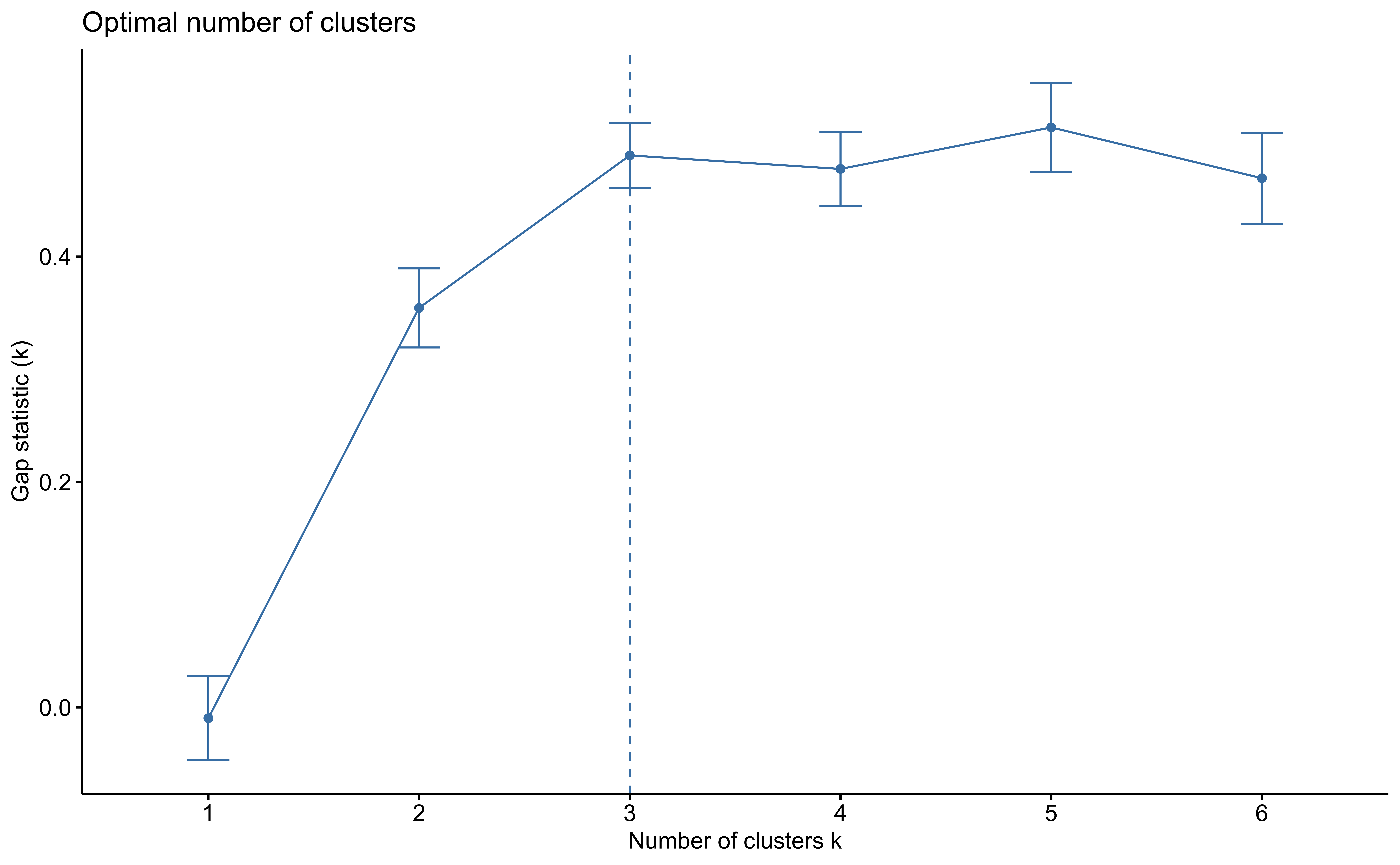
Choose K: Gap Statistics
Model-based Clustering
Gaussian Finite Mixture Models (GMM)
Assume each data point \(\mathbf{x}_i \in \mathbf{R}^p\) is generated from one of the \(K\) Gaussian distributions \(N(\boldsymbol \mu_k, \boldsymbol \Sigma_k)\), \(k = 1, \dots, K\).
Gaussian mixture model (GMM) has the form
\[p\left(\mathbf{x}_i\right) = \sum_{k=1}^K p_k N(\boldsymbol \mu_k, \boldsymbol \Sigma_k)\]
- GMM can be written as a latent variable model:
\[ \begin{align} \mathbf{x}_i \mid z_i &\sim N(\boldsymbol \mu_{z_i}, \boldsymbol \Sigma_{z_i})\\ z_i &\sim \text{Categorical}(p_1, \dots, p_K)\end{align}\]
- \(z_i \in \{1,2, \dots, K \}\) is the latent variable.
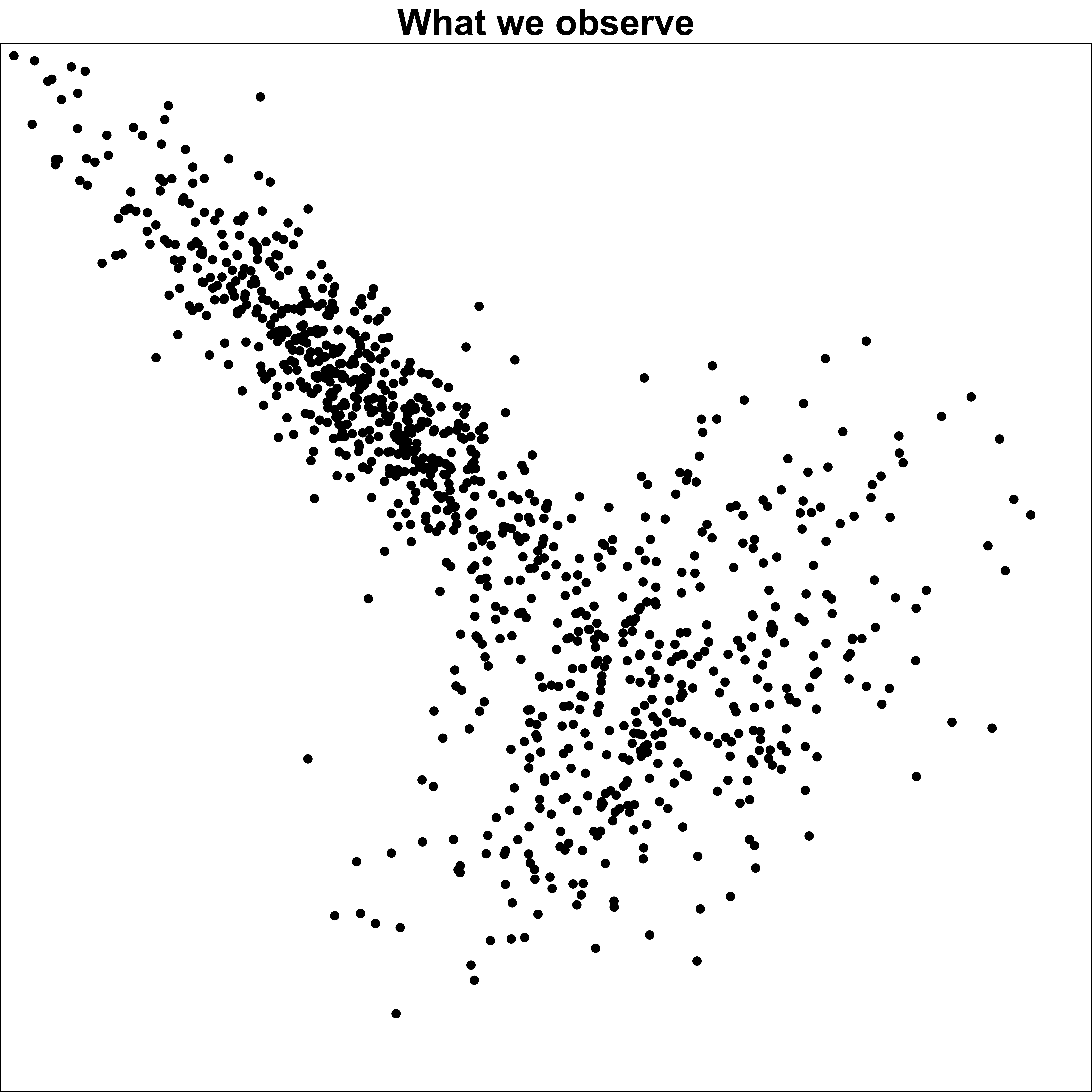
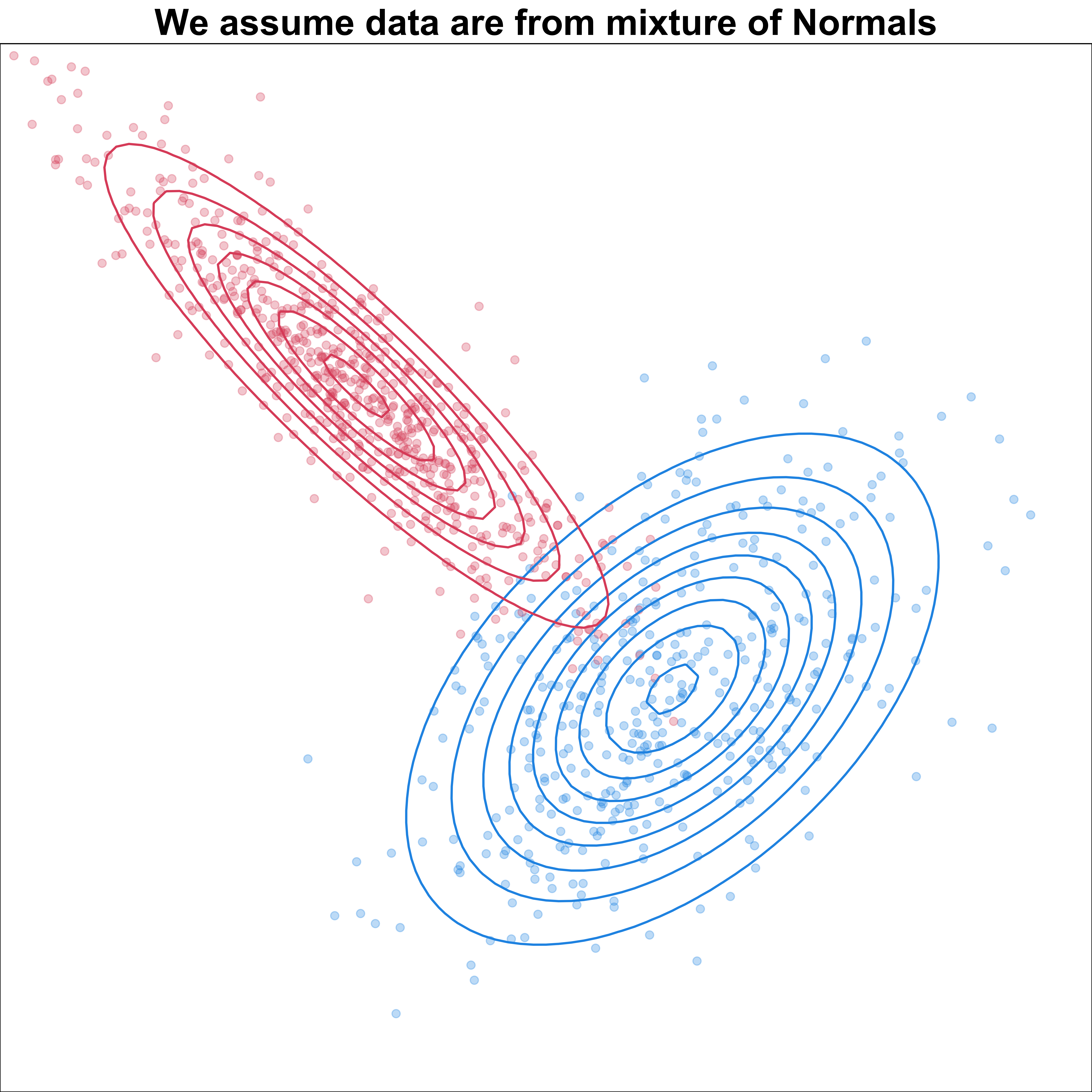
Mixture of Gaussians
\(p\left(\mathbf{x}_i\right) = (0.4) N(\boldsymbol \mu_1, \boldsymbol \Sigma_1) + (0.6)N(\boldsymbol \mu_2, \boldsymbol \Sigma_2)\), \(\boldsymbol \mu_1 = (1, -1)\); \(\boldsymbol \mu_2 = (-1.5, 1.5)\), \(\boldsymbol \Sigma_1 = \begin{bmatrix} 1 & 0.5 \\ 0.5 & 1 \end{bmatrix}\); \(\boldsymbol \Sigma_2 = \begin{bmatrix} 1 & -0.9 \\ -0.9 & 1 \end{bmatrix}\)
GMM for Clustering
Given the data and the model \[ \begin{align} \mathbf{x}_i \mid z_i &\sim N(\boldsymbol \mu_{z_i}, \boldsymbol \Sigma_{z_i})\\ z_i &\sim \text{Categorical}(p_1, \dots, p_K)\end{align},\] where \(\boldsymbol \theta= \{\boldsymbol \mu_{k}, \boldsymbol \Sigma_{k}, p_k \}_{k=1}^K\), we estimate the posterior probability that point \(i\) belongs to cluster \(k\): \[p\left(z_i = k \mid \mathbf{x}_i, \boldsymbol \theta\right),\] which is called the responsibility of cluster \(k\) for data point \(\mathbf{x}_i\).
With Bayes rule,
\[r_{ik} := p\left(z_i = k \mid \mathbf{x}_i, \boldsymbol \theta\right) = \frac{p\left(z_i = k \mid \boldsymbol \theta\right)p\left(\mathbf{x}_i \mid z_i = k , \boldsymbol \theta\right)}{\sum_{k'=1}^Kp\left(z_i = k' \mid \boldsymbol \theta\right)p\left(\mathbf{x}_i \mid z_i = k' , \boldsymbol \theta\right)} = \frac{p_kN(\boldsymbol \mu_{k}, \boldsymbol \Sigma_{k})}{\sum_{k'=1}^Kp_{k'}N(\boldsymbol \mu_{k'}, \boldsymbol \Sigma_{k'})}\]
- This procedure is called soft clustering.
Expectation-Maximization (EM) Algorithm
Gradient-based optimizers are hard to find a local minimum of the negative log likelihood (loss function) when there are unobserved latent variables in the model.
-
EM algorithm considers the complete data likelihood \(L(\mathbf{x}, \mathbf{z}\mid \boldsymbol \theta)\), and iteratively
- infers unobservable \(\mathbf{z}\) given \(\boldsymbol \theta\) (E-step)
- optimizes \(\boldsymbol \theta\) given the “filled in” data (M-step)
The complete data log likelihood is
\[\log L(\mathbf{x}, \mathbf{z}\mid \boldsymbol \theta) = \ell\left( \boldsymbol \theta\right):= \log \left[ \prod_{i=1}^np(\mathbf{x}_i, \mathbf{z}_i \mid \boldsymbol \theta)\right] = \sum_{i=1}^n \log p(\mathbf{x}_i, \mathbf{z}_i \mid \boldsymbol \theta)\]
- \(\ell\left( \boldsymbol \theta\right)\) cannot be computed since \(\mathbf{z}_i\) is unknown.
EM Algorithm
At iteration \(t\),
E-step: Take expectation w.r.t. \(\mathbf{z}_i \mid \mathbf{x}, \boldsymbol \theta^{(t-1)}\), or compute the expected complete data log likelihood \[Q\left(\boldsymbol \theta, \boldsymbol \theta^{(t-1)} \right) = \text{E}\left[\ell(\boldsymbol \theta) \mid \mathbf{x}, \boldsymbol \theta^{(t-1)} \right]\]
M-step: Maximize \(Q\left(\boldsymbol \theta, \boldsymbol \theta^{(t-1)} \right)\) w.r.t. \(\boldsymbol \theta\)
\[\boldsymbol \theta^{(t)} = \mathop{\mathrm{arg\,max}}_{\boldsymbol \theta} \, Q\left(\boldsymbol \theta, \boldsymbol \theta^{(t-1)} \right)\]
Stop until \(\|\boldsymbol \theta^{(t)} - \boldsymbol \theta^{(t-1)}\| < \epsilon\) or \(\|Q\left(\boldsymbol \theta^{(t)}, \boldsymbol \theta^{(t-1)} \right) - Q\left(\boldsymbol \theta^{(t-1)}, \boldsymbol \theta^{(t-1)} \right)\| < \epsilon\)
EM for GMM
\[\begin{align} Q\left(\boldsymbol \theta, \boldsymbol \theta^{(t-1)} \right) &= \text{E}\left[\ell(\boldsymbol \theta) \mid \mathbf{x}, \boldsymbol \theta^{(t-1)} \right] \\ &=\sum_{i=1}^n \text{E}\left[ \log \left[ \prod_{k=1}^K p_kp(\mathbf{x}_i \mid z_i, \boldsymbol \theta)^{I(z_i = k)}\right]\right]\\ &=\sum_{i=1}^n \sum_{k=1}^K \text{E}(I(z_i=k)) \log \left[p_kp(\mathbf{x}_i \mid z_i=k, \boldsymbol \theta) \right]\\ &=\sum_{i=1}^n \sum_{k=1}^K p\left(z_i = k \mid \mathbf{x}_i, \boldsymbol \theta\right) \log \left[p_kp(\mathbf{x}_i \mid z_i=k, \boldsymbol \theta) \right]\\ &=\sum_{i=1}^n \sum_{k=1}^K r_{ik} \log p_k + \sum_{i=1}^n \sum_{k=1}^K r_{ik} \log p(\mathbf{x}_i \mid z_i=k, \boldsymbol \theta)\end{align}\]
EM for GMM
\(\begin{align} Q\left(\boldsymbol \theta, \boldsymbol \theta^{(t-1)} \right)=\sum_{i=1}^n \sum_{k=1}^K r_{ik} \log p_k + \sum_{i=1}^n \sum_{k=1}^K r_{ik} \log p(\mathbf{x}_i \mid z_i=k, \boldsymbol \theta)\end{align}\)
- E-step:
\(r_{ik} = \frac{p_kN\left(\mathbf{x}_i \mid \boldsymbol \mu_{k}^{(t-1)}, \boldsymbol \Sigma_{k}^{(t-1)}\right)}{\sum_{k'=1}^Kp_{k'}N\left(\mathbf{x}_i \mid \boldsymbol \mu_{k'}^{(t-1)}, \boldsymbol \Sigma_{k'}^{(t-1)}\right)}\)
- M-step:
- \(p_k = \frac{\sum_{i=1}^n r_{ik}}{n}\)
- \(\boldsymbol \mu_k = \frac{\sum_{i=1}^n r_{ik}\mathbf{x}_i}{\sum_{i=1}^n r_{ik}}\)
- \(\boldsymbol \Sigma_k = \frac{\sum_{i=1}^n r_{ik}(\mathbf{x}_i - \boldsymbol \mu_k)(\mathbf{x}_i - \boldsymbol \mu_k)'}{\sum_{i=1}^n r_{ik}}\)
Set \(\boldsymbol \theta^{(t)} = \left(p_k, \boldsymbol \mu_k, \boldsymbol \Sigma_k \right)_{k=1}^K\) and return to the E-step.
EM and K-Means
-
In K-Means,
Assume \(p_k = 1/K\) and \(\boldsymbol \Sigma_k = \sigma^2\mathbf{I}\) are fixed.
E-step (hard EM/clustering):
\[p\left(z_i = k \mid \mathbf{x}_i, \boldsymbol \theta\right) \approx I(k = z_i^*),\] where \[z_i^* = \mathop{\mathrm{arg\,max}}_k \,\, p\left(z_i = k \mid \mathbf{x}_i, \boldsymbol \theta\right) = \mathop{\mathrm{arg\,min}}_k \,\, \|\mathbf{x}_i - \boldsymbol \mu_k\|^2\]
- M-step:
\[\boldsymbol \mu_k = \frac{\sum_{i:z_i = k}\mathbf{x}_i}{n_k},\] where \(n_k\) is the number of points belong to \(k\).
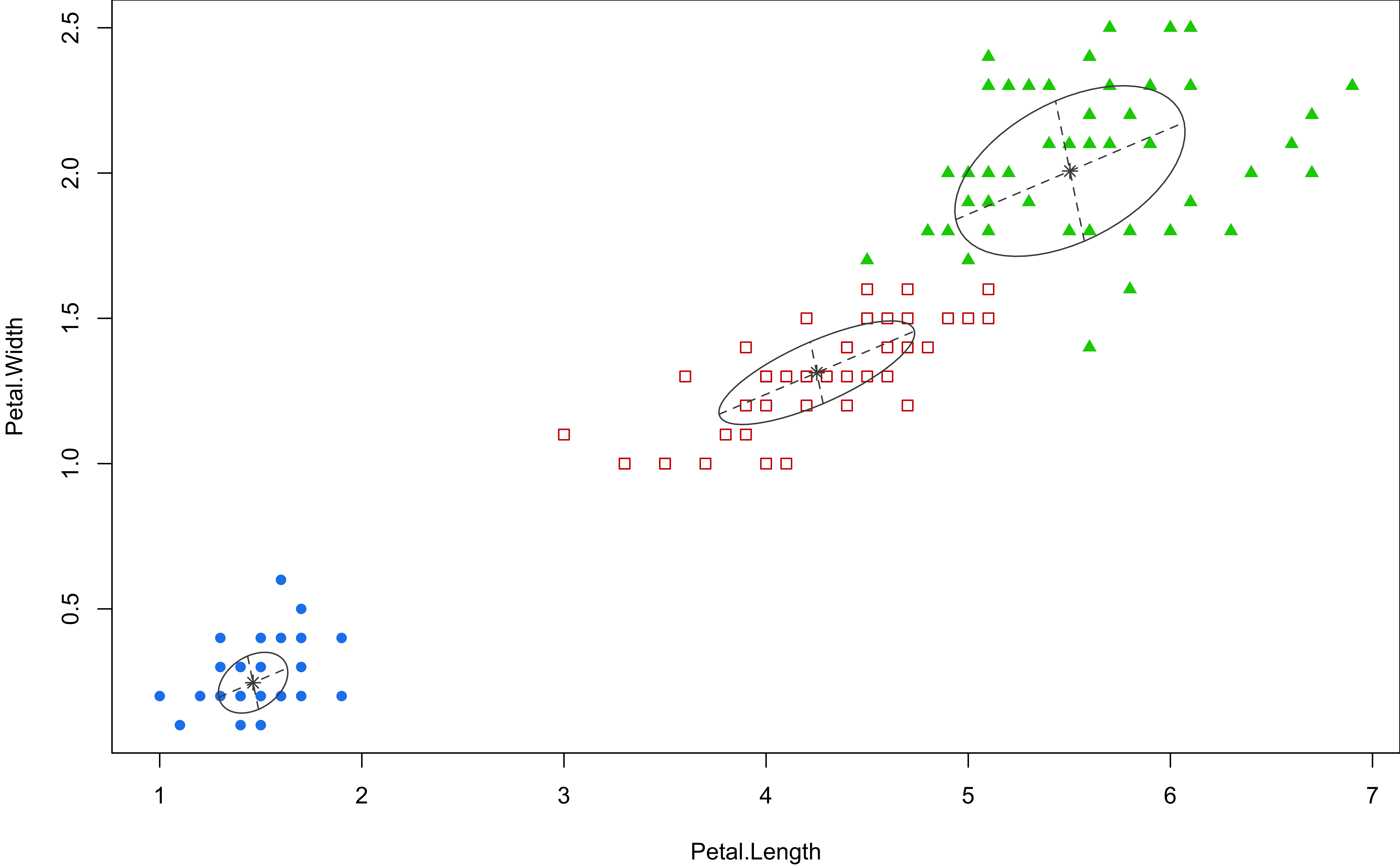
mclust
Other Topics
- Hierarchical Clustering
- Spectral Clustering
- Dirichlet Process Mixture Models