Artificial Neural Networks 🙌

MSSC 6250 Statistical Machine Learning

Dr. Cheng-Han Yu
Department of Mathematical and Statistical Sciences
Marquette University

Feed-forward Neural Networks

Neural Networks

• An (artifical) neural network is a machine learning model inspired by the biological neural networks that constitute animal brains.

Source: Wiki

Deep Learning

• A neural network takes an input vector of \(p\) variables \(X = (X_1, X_2, \dots, X_p)\) and builds a nonlinear function \(f(X)\) to predict the response \(Y\).

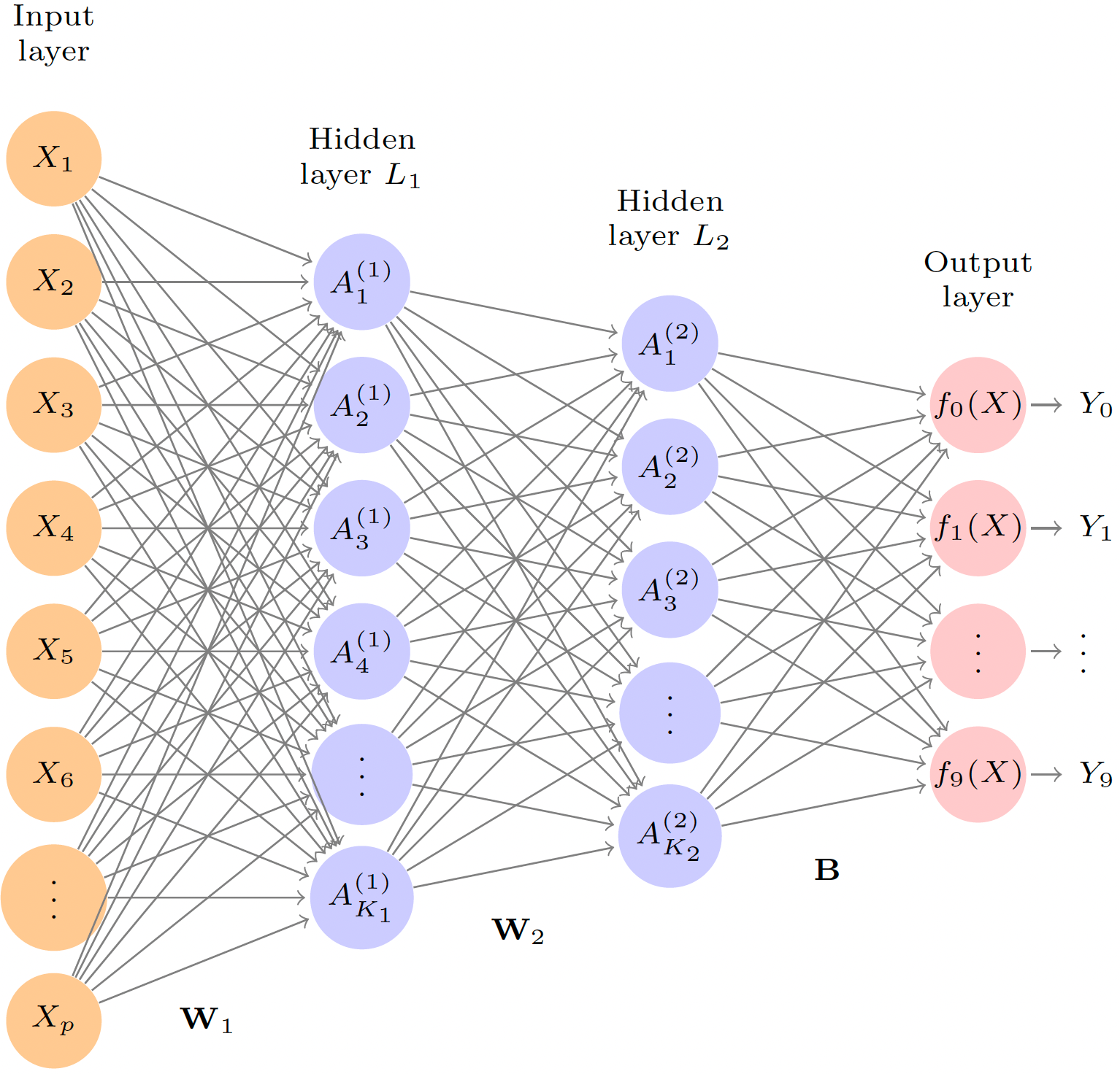
• A neural network with several hidden layers is called a deep neural network, or deep learning.

Source: ISL Ch 10

Source: http://brainstormingbox.org/a-beginners-guide-to-neural-networks/

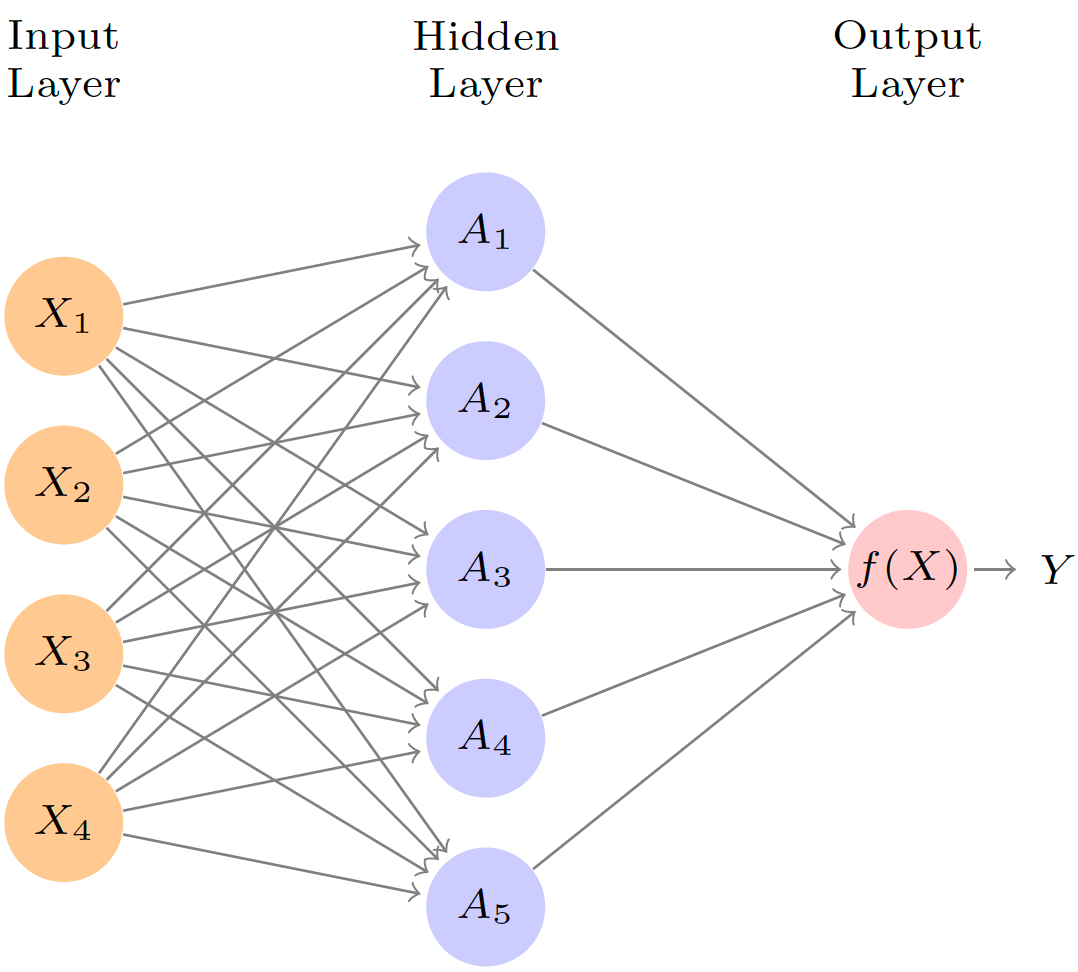
Single (Hidden) Layer Neural Network with One Output

Starts from inputs \(X\), for each hidden neuron \(A_k\), \(k = 1, \dots, K\),

• \(A_k(X) = g(w_{k0} + w_{k1}X_1 + \cdots + w_{kp}X_p)\)

• \(f(X) = g_f(\beta_0 + \beta_1A_1(X) + \cdots + \beta_KA_K(X))\)

• \(g_k(z)\) and \(g_f(z)\) are (non)linear activation functions that are specified in advance.

• \(\beta_0, \dots, \beta_K\) and \(w_{10}, \dots, w_{1p}, \dots, w_{K0}, \dots, w_{Kp}\) are parameters to be estimated.

• \(p = 4, K = 5\)

Source: ISL Fig. 10.1

We can think of each Ak as a different transformation hk(X) of the original function features, much like the basis functions

Linear Regression as Neural Network

Can we represent a linear regression model as a neural network?

• YES! Linear regression is a single layer neural network with

  • identity activation \(g(z) = z\) and \(g_f(z) = z\)
  • \(p = K\)
  • \(w_{kk} = 1\) and \(w_{kj} = 0\) for all \(k \ne j\)

https://ml-explained.com/blog/kernel-pca-explained

Logistic Regression as Neural Network

Can we represent a binary logistic regression model as a neural network?

• YES! Binary logistic regression is a single layer neural network with

  • identity activation \(g(z) = z\)
  • sigmoid activation \(g_f(z) = \frac{e^{z}}{1+e^z}\)
  • \(p = K\)
  • \(w_{kk} = 1\) and \(w_{kj} = 0\) for all \(k \ne j\)

Activation Functions

Activation functions are usually continuous for optimization purpose.

• sigmoid: \(\frac{1}{1+e^{-z}} = \frac{e^z}{1+e^z}\)
• hyperbolic tangent: \(\frac{e^z - e^{-z}}{e^z + e^{-z}}\)
• rectified linear unit (ReLU): \(\max(0, z)\); \(\ln(1 + e^z)\) (Soft version)
• Gaussian-error linear unit (GELU): \(z \Phi(z)\), where \(\Phi(\cdot)\) is the \(N(0, 1)\) CDF

Choose a Activation Function

• The activation function used in hidden layers is typically chosen based on the type of neural network architecture.

  • Multilayer Perceptron (MLP): ReLU (leaky ReLU)
  • Convolutional Neural Network: ReLU
  • Recurrent Neural Network: Tanh and/or Sigmoid

• never use softmax and identity functions in the hidden layers.

• For output activation function,

  • Regression: One node, Linear
  • Binary Classification: One node, Sigmoid
  • Multiclass Classification: One node per class, Softmax
  • Multilabel Classification: One node per class, Sigmoid

Finally, we make an remark that a single hidden layer neural network is sufficient for approximating any continuous function - https://machinelearningmastery.com/choose-an-activation-function-for-deep-learning/ - https://towardsdatascience.com/how-to-choose-the-right-activation-function-for-neural-networks-3941ff0e6f9c

When to Use Deep Learning

• The signal to noise ratio is high.

• The sample size is huge.

• Interpretability of the model is not a priority.

• When possible, try the simpler models as well, and then make a choice based on the performance/complexity tradeoff.

• Occam’s razor principle: when faced with several methods that give roughly equivalent performance, pick the simplest.

Fitting Neural Networks

Source: ISL Fig. 10.1

\[\min_{\boldsymbol \beta, \{\mathbf{w}\}_1^K} \frac{1}{2}\sum_{i=1}^n\left(y_i - f(x_i) \right)^2,\] where \[f(x_i) = \beta_0 + \sum_{k=1}^K\beta_Kg\left( w_{k0} + \sum_{j=1}^pw_{kj}x_{xj}\right).\]

• This problem is difficult because the objective is non-convex: there are multiple solutions.

Gradient Descent

• For the objective function \(R(\theta)\) and the parameter vector \(\theta\) to be estimated, gradient descent keeps finding new parameter value that reduces the objective until the objective fails to decrease.

• \(\theta^{(t+1)} = \theta^{(t)} -\rho\nabla R(\theta^{(t)})\), where \(\rho\) is the learning rate that is typically small like 0.001.

• \(\nabla R(\theta^{(t)}) = \left. \frac{\partial R(\theta)}{\partial \theta} \right \rvert_{\theta = \theta^{(t)}}\)

Backpropagation

\[\begin{align} R(\theta) \overset{\triangle}{=} \sum_{i=1}^nR_i(\theta) =& \frac{1}{2}\sum_{i=1}^n \big(y_i - f_{\theta}(x_i)\big)^2\\ =& \frac{1}{2} \sum_{i=1}^n \big(y_i - \beta_0 - \beta_1 g(w_1' x_i) - \cdots - \beta_K g(w_K' x_i) \big)^2 \\ \end{align}\]

• Nothing but chain rule for differentiation:

With \(z_{ik} = w_k' x_i\),

\[\frac{\partial R_i(\theta)}{\partial \beta_{k}} = \frac{\partial R_i(\theta)}{\partial f_{\theta}(x_i)} \cdot \frac{\partial f_{\theta}(x_i)}{\partial \beta_{k}} = {\color{red}{-\big( y_i - f_{\theta}(x_i)\big)}} \cdot g(z_{ik})\]

\[\frac{\partial R_i(\theta)}{w_{kj}} = \frac{\partial R_i(\theta)}{\partial f_{\theta}(x_i)} \cdot \frac{\partial f_{\theta}(x_i)}{\partial g(z_{ik})} \cdot \frac{\partial g(z_{ik})}{\partial z_{ik}} \cdot \frac{\partial z_{ik}}{\partial w_{kj}} = {\color{red}{-\big( y_i - f_{\theta}(x_i)\big)}} \cdot \beta_k \cdot g'(z_{ik}) \cdot x_{ij}\]

• Reuse the red part in different layers of gradients to reduce computational burden.

Other Topics

• Stochastic Gradient Descent

• Dropout Learning

• Convolutional Neural Network (Spatial modeling)

• Recurrent Neural Network (Temporal modeling)

• Bayesian Deep Learning

https://stackoverflow.com/questions/70977755/could-not-find-a-version-that-satisfies-the-requirement-tensorflow-python3-9-6 https://developer.apple.com/metal/tensorflow-plugin/